Unemployment and Inflation
Of all of the measures of the health of an economy, the two that seem to get the most attention are the unemployment rate and the inflation rate. In this lesson, we will look at both measures, show how they are defined and calculated, and explain their importance. Throughout the remainder of the course, the impact on the unemployment rate and the inflation rate will be key considerations in evaluating the wisdom of particular economic policies. The fundamental understanding that you gain of these two variables in this lesson, therefore, must be retained for the rest of the course.
Section 01: Unemployment Data
Before giving the exact formula for the unemployment rate and letting you calculate it, let’s define a few useful terms:
Civilian non-institutional population: Persons 16 years of age and older residing in the 50 states and the District of Columbia, who are not inmates of institutions (e.g., penal and mental facilities, homes for the aged), and who are not on active duty in the Armed Forces. (238,889,000 in December 2010.)
Civilian labor force: All persons in the civilian non-institutional population classified as either employed or unemployed. (153,156,000 in December 2010.)
Employed persons: All persons who, during the reference week (week including the twelfth day of the month), (a) did any work as paid employees, worked in their own business or profession or on their own farm, or worked 15 hours or more as unpaid workers in an enterprise operated by a member of their family, or (b) were not working but who had jobs from which they were temporarily absent. Each employed person is counted only once, even if he or she holds more than one job. (139,159,000 in December 2010.)
Unemployed persons: All persons who had no employment during the reference week, were available for work, except for temporary illness, and had made specific efforts to find employment some time during the 4 week-period ending with the reference week. Persons waiting to be recalled to jobs from which they were laid off are still counted as unemployed; one needn’t be looking for work to be classified as unemployed. (13,997,000 in December 2010.)
Notice that by these definitions, the Labor Force includes both the employed and the unemployed. To be considered unemployed you must be looking for work or about to return to a job. Otherwise, you are NOT IN THE LABOR FORCE. In December 2010, 85,733,000 persons in the United States were not in the labor force! Of those, according to the Current Population Survey, 6,212,000 wanted a job but had quit looking because they became discouraged by not being able to find one. These are sometimes referred to as discouraged “workers,” but are not counted as being part of the labor force, because they do not have a job and are no longer looking.
The Unemployment Rate
The unemployment rate is equal to the number of people unemployed divided by the number of people in the civilian labor force times 100. We multiply times 100 so that the rate can be expressed as a percent:
UR = (Unemployed/Civilian Labor Force) X 100
With the above data for December 2010, let me demonstrate calculating the unemployment rate:
UR = (13,997,000/153,156,000) X 100 = 9.139%
The unemployment rate in December 2010 in the United States was approximately 9.14%.
Based on the data given below for the entire year 2010 (the monthly average), calculate the unemployment rate for the United States for 2010.
| Civilian Non-Institutional Population | 237,830,000 |
| Civilian Labor Force | 153,889,000 |
| Employed | 139,064,000 |
| Unemployed | 14,825,000 |
| Not in the Labor Force | 83,941,000 |
Types of Unemployment
Not everyone who is unemployed is unemployed for the same reasons. Generally economists classify unemployment into three different types: Frictional, Structural, and Cyclical.
Frictional Unemployment is a temporary, usually very short term, type of unemployment. It is sometimes referred to as the worker simply being “between jobs.” Even in a very healthy economy, there will always be some unemployment of this type. A worker may get frustrated with a boss and quit his job, only to find a new one two weeks later. For that short duration, he is unemployed. A student may graduate from college in the spring and wait to begin looking for a job until after graduation. During his job search he is unemployed, but in a healthy economy he may find a job within a month. He is unemployed during that month, but that is fairly short. Because Frictional Unemployment is usually resolved quickly, it is not seen as a serious problem and generally does not elicit a government reaction.
Structural Unemployment is unemployment due to a mismatch between the structure of the economy and the skills of the workers. Let’s say you had an economy with 1,000 workers who were unemployed and in which there were 1,000 jobs available. If the skills of the workers did not meet the needs of the employers, then those unemployed workers would remain unemployed even in the face of 1,000 available jobs. This is a much more serious form of unemployment than Frictional Unemployment, because its solution is not likely to be found without retraining or reeducating the unemployed workers. Structural Unemployment, therefore, is likely to persist for much longer periods of time, and in extreme situations may not be resolved for an individual until he reaches the age of retirement.
In the late 1970s and early 1980s the United States experienced a change in the structure of our economy as multiple steel mills shut down across the North-central and Northeast United States. The loss of jobs on the part of the steel workers during this time period was not a temporary phenomenon. Their jobs had permanently disappeared as the automobile industry, one of the largest consumers of steel, changed the way they produced cars. Large heavy cars were replaced by smaller, lighter-weight cars for fuel efficiency considerations. The United States faced a situation where a large number of men, some of whom were well into the second half of their working lives, lost their jobs in the only industry for which they had marketable skills. The fact that at this same time there were many jobs available in Silicon Valley California was not a comfort to these unemployed workers. Their skills did not match the needs of the high-tech employers in California and the geographical mismatch only added to the problem. Only an aggressive retraining program would have made these unemployed steel workers employable in another sector.
The third type of unemployment that we experience in our economy is called Cyclical Unemployment. All economies experience what is called a business cycle. Remember from the previous lesson on the Gross Domestic Product that we use the real GDP to measure growth in the economy. When an economy is experiencing a multi-quarter gain in the real GDP the economy is said to be in a boom cycle. This period of expansion may eventually peak and be followed by a multi-quarter decline in the real GDP called a recession. During a recession, the falling output is generally accompanied by layoffs for employees. The resulting unemployment is called Cyclical Unemployment, because it is associated with the business cycle described above. Recessions vary in their length, but eventually the economy tends to hit bottom, called a trough, and then another boom cycle begins. It is important to note that the long run trend in the economy may be upward even though there are short run recessions and booms. When the economy hits a trough and begins to go into another boom cycle, initially the upward movement can be thought of as a recovery until the economy gets back to the same level of output as the former peak. Once that level is achieved, any additional boom may be thought of as economic growth until a new, higher peak is reached. To the extent that a boom consists of both a recovery and addition growth, the trend of the economy is upward. During the boom cycles, unemployed workers are called back to work and the Cyclical Unemployment is eliminated as the economy heads towards its next peak.
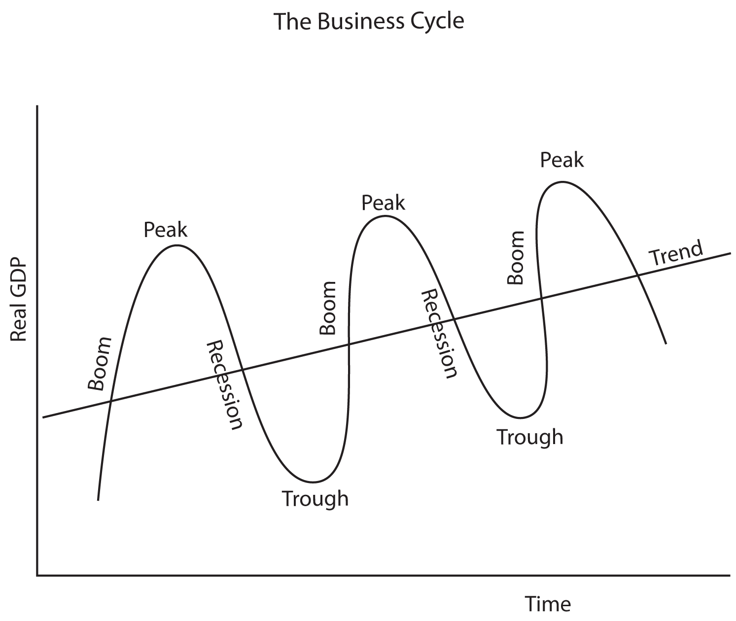
When the economy is at its peak there will be no Cyclical Unemployment, though Frictional and Structural Unemployment may still exist. The rate of unemployment in an economy when there is NO Cyclical Unemployment (in other words when the economy is very healthy and producing at its full capacity) is called the Natural Rate of Unemployment, or sometimes the Full-Employment level of Unemployment.
Because Cyclical Unemployment occurs as a result of the business cycle, the government will often try to intervene by institute policies to reduce the severity or duration of a recession, or to sustain an expansion. Cyclical Unemployment can be severe in the case of prolonged recessions, but does not necessarily have to be accompanied by thoughts of retraining, additional education, or changing careers. At the end of most recessions, cyclically unemployed workers go back to their same or very similar jobs. The potential GDP of the economy is the amount we can produce when we are at full employment or at the Natural Rate of Unemployment. It can be thought of as the output of the economy when we are at a peak. The difference between the potential GDP and the actual GDP is called the GDP Gap. This gap represents the lost output that results from operating at less than full employment, and is sometimes used to measure a recession’s impact on the economy. The relationship between Cyclical Unemployment and the GDP Gap is demonstrated by Okun’s Law.
Because most laws in economics are based on economic theory and Okun’s Law is based on Arthur Okun’s empirical observations during the 1950s and 1960s, it might be suggested that Okun’s Law is not a law at all, but more of a “rule of thumb.”
Demographic Differences in Unemployment Rates
While we normally report the unemployment rate for the economy as a whole, it is important to note that unemployment effects different demographic groups at different rates. So while US the unemployment rate in December 2010 was 9.4% overall, consider the differences in unemployment rates for the demographic groups listed below:
| Workers with less than a High School diploma | 14.9% |
| Workers with a High School diploma | 10.3% |
| Workers with Some College Education | 8.4% |
| Workers with a Bachelor’s Degree | 4.7% |
| Adults aged 20 and over | 8.9% |
| Teenagers aged 16–19 | 25.9% |
| Blacks | 16% |
| Whites | 8.7% |
| Asians | 7.5% |
| Men | 10.5% |
| Women | 8.6% |
You can see that unemployment is not distributed uniformly across all segments of our population!
Return to the course in I-Learn and complete the activity that corresponds with this material.
Section 02: Inflation
As stated earlier, besides the unemployment rate, another measure of the health of the economy is the inflation rate. Inflation is the rise in the average price level in the economy. The rate of inflation is the rate of change in the price level. The inflation rate can be measured by the following formula:
Where P1 is the average price level this year and P0 is the average price level last year.
It is easy to see that if the price level this year is higher than the price level last year inflation is going to be positive. Though it is uncommon, it is also possible to have the average price level in the economy fall. This is called deflation and using the above formula you would get a negative inflation rate. There was a small amount of deflation in 2009 when the inflation rate was -0.4%. The last time there was deflation prior to 2009 was 1955! Inflation can vary in its severity from low (low single digits) levels of inflation to hyperinflation (5 to 6 digit and more!).
The Consumer Price Index
One common measure of inflation in the United States is called the consumer price index or the CPI. If you hear the inflation rate reported in the media, you are generally hearing the latest estimate of the CPI. The CPI is calculated as follows:
The fixed basket of goods that they use to calculate the CPI is composed of 300 consumer goods and services purchased by a typical urban consumer. The prices of these goods are collected each month by the Bureau of Labor Statistics (BLS) by economic analysts from all over the country. Over 80,000 individual items are priced each month. Weights are applied to prices depending on the population of the area from which the price is collected. Therefore, the price of a tube of toothpaste in Los Angeles is given more weight than the price of the same tube of toothpaste in Idaho Falls. For additional information on how the CPI is calculated and what is contained in the “market basket of goods” used by the BLS to measure the CPI, see http://www.bls.gov/cpi/cpifaq.htm.
On average, when the prices of goods goes up the CPI will indicate that inflation has occurred in the economy and on average when prices have fallen the CPI will indicate deflation. In looking at the formula for the CPI, you will note that it is an index that will be equal to 100 if the prices of goods and services have remained the same from one time period to the next. So if the index is 100, it is the base period and you calculate a CPI of 103 in the current period, then you could say that there has been 3% inflation since the base period. If the CPI is equal to 99 in the current period then you could say there has been 1% deflation since the base period. What if the CPI were 100 in 2002, 112.5 in 2006, and 121.5 in 2010? Let’s see if we can calculate inflation rates between these various years. Between 2002 and 2006 is easy because 2002 is the base year and has a CPI of 100. Since the CPI was 112.5 in 2006 we would simply say that there was 12.5% inflation between 2002 and 2006. But how much inflation occurred between 2006 and 2010? To be able to express the inflation rate as a percent, we must use the formula for an inflation rate given above:
Notice that the CPI changed by 9 index points (121.5–112.5 = 9), but only by 8 percentage points. Inflation is always measured by percentage changes in prices, not simply by changes in the index points.
Think About It: Inflation Rate
From the official statistics of the United States we find that the CPI in 1983 was 100; in 1987 it was 113.6, and in 1993 it was 144.5. What was the inflation rate between 1984 and 1987? What was the inflation rate between 1987 and 1993? Did prices rise per year on average at a faster rate from 1983 to 1987, or from 1987 to 1993?
Some Impacts of Inflation on the Economy
Let’s look at some of the impacts of inflation on the economy. First, an issue that is important to every worker in the United States is the impact of inflation on their income. Let’s say that you earn $100,000 a year in income and that you do not receive a pay raise from one year to the next. If there has been 4% inflation during that time period, then you have actually received a 4% pay cut! Why? Because, if your pay remains the same and prices go up by 4%, then your income will buy 4% less next year than it bought the year before. Your nominal income has stayed the same but your REAL income has fallen. We can generally say that, in terms of pay increases, your increase in real income is equal to the increase in your nominal income minus the inflation rate.
Think About It: Inflation’s Effect on Real Income
Answer the following questions:
1. If you get a 5% increase in your nominal income in a year when the economy experiences 2% inflation, how much has your real income gone up?
2. If you get a 5% increase in your nominal income in a year when the economy experiences 5% inflation, how much has your real income gone up by?
3. If you get a 5% increase in your real income in a year when the economy experiences 5% inflation, how much must your nominal income have gone up by?
4. If you feel like you have done a great job this year and you want to negotiate a 7% pay raise with your employer—and you think inflation is going to be 3%—how much of a pay raise should you ask for?
A second impact that inflation can have on the economy is to redistribute income and wealth, either from creditors to debtors if the inflation is not correctly anticipated, or from one sector of the economy to another if the inflation is not balanced. Let’s look at each of these cases individually.
If you were a banker and wanted to make a one-year loan to someone, from which you would earn 4% interest, what interest rate would you charge if you thought the inflation rate was going to be 2% next year? You would charge the borrower an interest rate of 6% (the nominal interest rate) so that you would earn 4% real interest. This is because the borrower would be paying you back with money that is worth 2% less than the money he or she borrowed (that’s the impact of 2% inflation!). What if you do not anticipate inflation correctly? In this example, what is the impact on the creditor (the banker) if he thinks the inflation rate is going to be 2% and it actually turns out to be 5%? If he makes the loan at a 6% nominal interest rate and there is 5% inflation, then the real rate of interest that he will earn is only 1%, far below the 4% he wanted to earn.
Important Note: In the previous paragraph, you have learned an important concept in economics—the difference between a nominal variable and a real variable. A real variable always takes into account the impact of inflation on the nominal variable. The word nominal comes from a Latin word meaning “named.” So the nominal interest rate is the “named” interest rate, or the interest rate that is quoted by the bank. The real interest rate, on the other hand, is the actual interest rate that ends up being paid after the impact of inflation is taken into account. The relationship is as follows:
Real Interest = Nominal Interest – Inflation Rate.
Thus, if inflation is unanticipated or anticipated incorrectly, wealth is transferred from the creditor to the debtor. In general, because inflation is difficult to anticipate, debtors like inflation and creditors do not.
Next let’s look at the issue of whether inflation is “balanced.” If we say that inflation last year was 4%, you might imagine that the price of everything went up 4%. That would be balanced inflation. But the reality would be that the prices of some things went up 4%, the prices of other things went down, and the prices of some items might have gone up by far more than 4%. We only know that price went up on average by 4%. So let’s say that the prices of food in grocery stores go up by 2% and the prices of meals at restaurants go up by 8%. Consumers might be led to buy relatively more food at the grocery store and eat at restaurants less often. This unbalanced inflation would redistribute wealth from restaurant owners to grocery store owners. If inflation is balanced, no such redistribution would take place.
The Relationship between Inflation and Unemployment
Over some short periods of time, we may observe an inverse relationship between unemployment and inflation. That is to say that during periods of high unemployment, inflation may be relatively low; during periods of high inflation, unemployment may be relatively low. This inverse relationship can be illustrated by what has come to be known as the Phillips Curve, shown below.
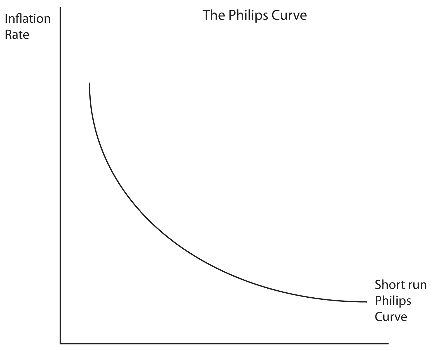
Named for New Zealand economist William Phillips, the Phillips Curve is no longer widely used because it is too simplistic. In fact, looking at US data, no single Phillips Curve can be distinguished over the time period from 1960 to 2010. Over shorter time periods, some groupings of data have a general downward slope, but at very different levels, suggesting that the Phillips Curve shifts at times and that the relationship suggested by Phillips does not hold over time.