Supply and Demand
Teach a parrot the terms of 'supply and demand' and you’ve got an economist.
-- Thomas Carlyle
A market brings together and facilitates trade between buyers and sellers of a good or services. These markets range from bartering in street markets to trades that are made through the internet with individuals around the world that never have met face to face.
A market consists of those individuals who are willing and able to purchase the particular good and sellers who are willing and able to supply the good. The market brings together those who demand and supply the good to determine the price.
For example, the number of many apples an individual would be willing and able to buy each month depends in part on the price of apples. Assuming only price changes, then at lower prices, a consumer is willing and able to buy more apples. As the price rises (again holding all else constant), the quantity of apples demanded decreases. The Law of Demand captures this relationship between price and the quantity demanded of a product. It states that there is an inverse (or negative) relationship between the price of a good and the quantity demanded.
Recall, that we represent economic laws and theory using models; in this case we can use a demand schedule or a demand curve to illustrate the Law of Demand. The demand schedule shows the combinations of price and quantity demanded of apples in a table format. The graphical representation of the demand schedule is called the demand curve.
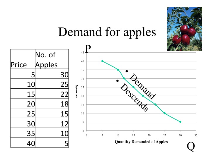
When graphing the demand curve, price goes on the vertical axis and quantity demanded goes on the horizontal axis. A helpful hint when labeling the axes is to remember that since P is a tall letter, it goes on the vertical axis. Another hint when graphing the demand curve is to remember that demand descends.
The demand curve reflects our marginal benefit and thus our willingness to pay for additional amounts of a good. It makes sense that our marginal benefit, or willingness to pay for a good, would decline as we consume additional units because we get less additional satisfaction from each successive unit consumed. For example, at lunch time you decide to buy pizza by-the-piece. You'd be willing to pay a lot for that first piece to satisfy your hunger. But what about the second piece? Perhaps a little less. If we keep considering each additional piece, we might ask what the 3rd, 4th or 5th piece is worth to you. By that point, you'd be willing to pay less, perhaps much less. The law of demand and our models illustrate this behavior.
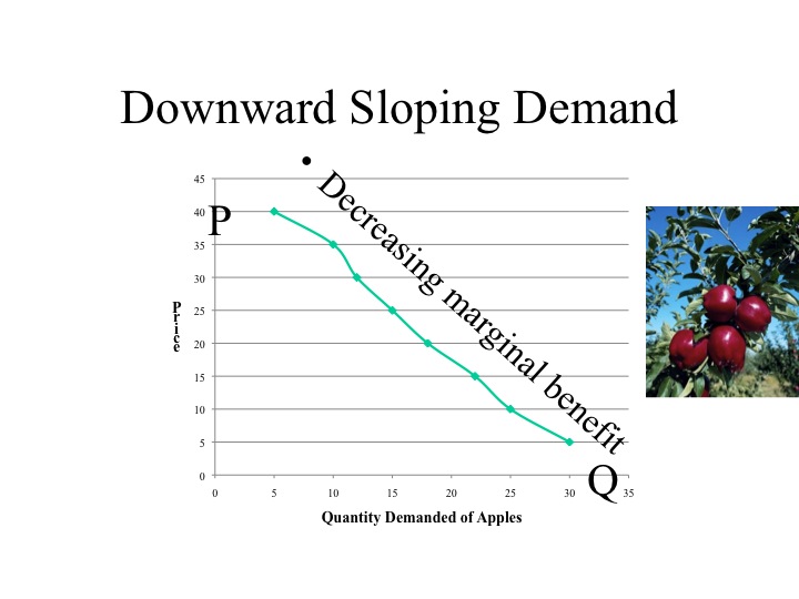
A more formal examination of the law of demand shows the most basic reasons for the downward sloping nature of demand. The first is the substitution effect which states that as the price of the good declines, it becomes relatively less expensive compared to the price of other goods and thus the quantity demanded is greater at a lower price. When the price of the good rises, the opposite occurs; that is, as the price of the good becomes relatively more expensive compared to other goods a lower quantity will be demanded. For example, as the price of apples increases or decreases, apples become relatively more or less expensive compared to other goods, such as oranges. Thus if the price of apples declines, consumers will buy more apples since they are relatively less expensive compared to other goods, such as oranges.
The second factor is the income effect which states that as the price of a good decreases, consumers become relatively richer. Now, their incomes have not increased, but their buying power has increased due to the lower price. If they continued to buy the same amount, they would have some money left over - some of that extra money could be spent on the good that has the lower price, that is quantity demanded would increase. On the other hand, as the price of a good increases, then the buying power of individuals decreases and the quantity demanded decreases. For example, at 20 cents per apple, we are able to purchase 5 apples for $1 but if the price falls to 10 cents, we would be able to buy 10 apples for $1. Although our income has not changed, we have become relatively richer.
At this point, we have explained why there is an inverse relationship between price and quantity demanded (i.e. we've explained the law of demand). The changes in price that we have discussed cause movements along the demand curve, called changes in quantity demanded. But there are factors other than price that cause complete shifts in the demand curve which are called changes in demand (Note that these new factors also determine the actual placement of the demand curve on a graph).
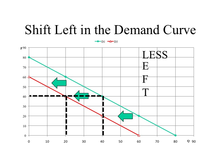
While a change in the price of the good moves us along the demand curve to a different quantity demanded, a change or shift in demand will cause a different quantity demanded at each and every price. A rightward shift in demand would increase the quantity demanded at all prices compared to the original demand curve. For example, at a price of $40, the quantity demanded would increase from 40 units to 60 units. A helpful hint to remember that more demand shifts the demand curve to the right.
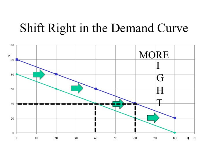
A leftward shift in demand would decrease the quantity demanded to 20 units at the price of $40. With a decrease in demand, there is a lower quantity demanded at each an every price along the demand curve.
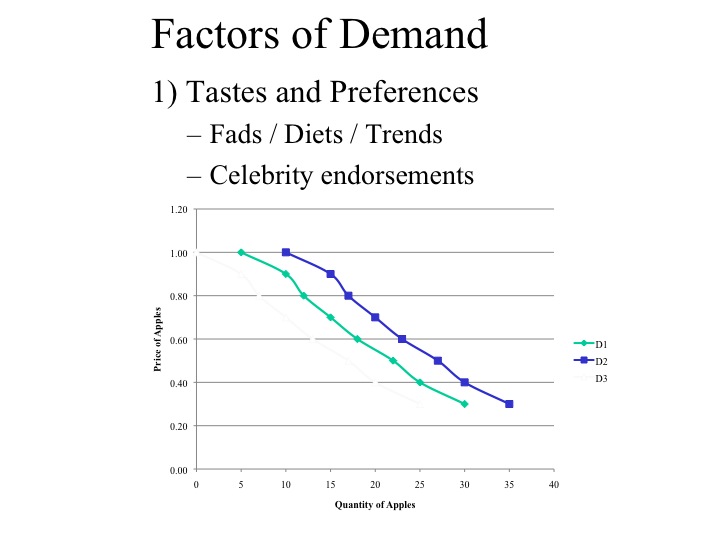
A change in tastes and preferences will cause the demand curve to shift either to the right or left. For example, if new research found that eating apples increases life expectancy and reduces illness, then more apples would be purchased at each and every price causing the demand curve to shift to the right. Companies spend billions of dollars in advertising to try and change individuals’ tastes and preferences for a product. Celebrities or sports stars are often hired to endorse a product to increase the demand for a product. A leftward shift in demand is caused by a factor that adversely effects the tastes and preferences for the good. For example, if a pesticide used on apples is shown to have adverse health effects.
Another factor that determines the demand for a good is the price of related goods. These can be broken down into two categories – substitutes and complements. A substitute is something that takes the place of the good. Instead of buying an apple, one could buy an orange. If the price of oranges goes up, we would expect an increase in demand for apples since consumers would move consumption away from the higher priced oranges towards apples which might be considered a substitute good. Complements, on the other hand, are goods that are consumed together, such as caramels and apples. If the price for a good increases, its quantity demanded will decrease and the demand for the complements of that good will also decline. For example, if the price of hot dogs increases, one will buy fewer hot dogs and therefore demand fewer hot dog buns, which are complements to hot dogs.
Remember that demand is made up of those who are willing and able to purchase the good at a particular price. Income influences both willingness and ability to pay. As one’s income increases, a person's ability to purchase a good increases, but she/he may not necessarily want more. If the demand for the good increases as income rises, the good is considered to be a normal good. Most goods fall into this category; we want more cars, more TVs, more boats as our income increases. As our income falls, we also demand fewer of these goods. Inferior goods have an inverse relationship with income. As income rises we demand fewer of these goods, but as income falls we demand more of these goods. Although individual preferences influence if a good is normal or inferior, in general, Top Ramen, Mac and Cheese, and used clothing fall into the category of an inferior good.
Another factor of demand is future expectations. This includes expectations of future prices and income. An individual that is graduating at the end of the semester, who has just accepted a well paying job, may spend more today given the expectation of a higher future income. This is especially true if the job offer is for more income than what he had originally anticipated. If one expects the price of apples to go up next week, she will likely buy more apples today while the price is still low.
The last factor of demand is the number of buyers. A competitive market is made up of many buyers and many sellers. Thus a producer is not particularly concerned with the demand of one individual but rather the demand of all the buyers collectively in that market. As the number of buyers increases or decreases, the demand for the good will change.
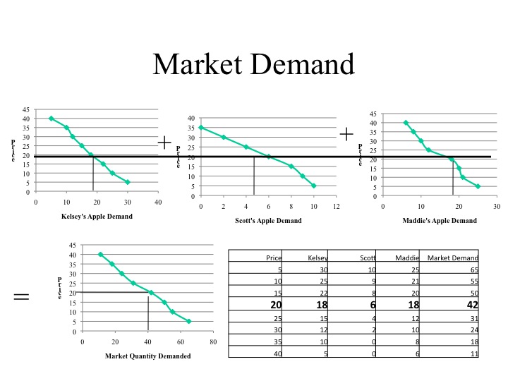
The market demand is determined by the horizontal summation of the individual demands. For example, at 20 cents per apple, Kelsey would buy 18 apples, Scott would buy 6 and Maddie would buy 18, making the market quantity demanded at 20 cents equal to 42 apples.
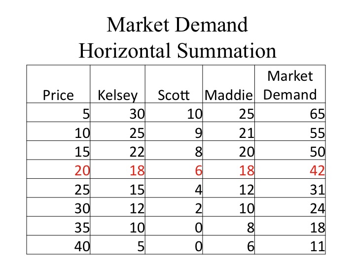
When determining the market demand graphically, we select a price then find the quantity demanded by each individual at that price. To determine the entire demand curve, we would then select another price and repeat the process.
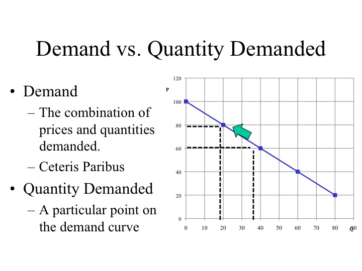
At this point, it is important to re-emphasize that there is an important distinction between changes in demand and changes in quantity demanded. The entire curve showing the various combinations of price and quantity demanded represents the demand curve. Thus a change in the price of the good does not shift the curve (or change demand) but causes a movement along the demand curve to a different quantity demanded. If the price returned to its original price, we would return to the original quantity demanded.
If the price were originally $60, the quantity demanded would be 40 units. An increase in the price of the good to $80 decreases the quantity demanded to 20 units. This is a movement along the demand curve to a new quantity demanded. Note that if the price were to return to $60, the quantity demanded would also return to the 40 units.
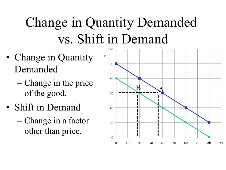
A shift or change in demand comes about when there is a different quantity demanded at each price. At $60 we originally demanded 40 units. If there is a lower quantity demanded at each price, the demand curve has shifted left. Now at $60, there are only 20 units demanded. Shifts in demand are caused by factors other than the price of the good and, as discussed, include changes in: 1) tastes and preferences; 2) price of related goods; 3) income; 4) expectations about the future; and 5) market size.
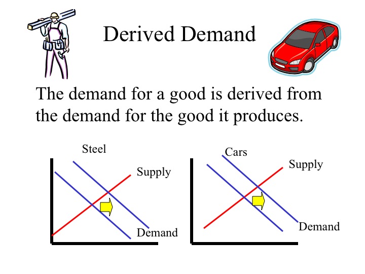
The demand for an input or resource is derived from the demand for the good or service that uses the resource. We do not value steel in and of itself, but since we demand cars, we indirectly demand steel. If the demand for cars increases, this would cause an increase in the demand for the steel that is used to make the cars.
Practice
Identify how each of the following would change the demand (shift right, shift left, move along).
| Market | Item |
| 1. Oranges | A new diet consisting of eating six oranges a day becomes the latest diet fad. |
| 2. Cars | Consumers’ income rises. |
| 3. Cars | The price of gasoline doubles. |
| 4. Gym memberships | The price of personal exercise equipment increases. |
| 5. Shoes | The number of shoe manufacturers increases. |
| 6. Arthritis medication | The number of elderly citizensincreases. |
Answers: 1. D-right 2. D-right 3. D-left 4. D-right 5. Along 6. D-right
Supply
Supply shows the amount that producers are willing and able to supply to the market at each given price. Producers must receive a price that covers the marginal cost of production. As the price of the good rises, producers are willing to produce more of the good even though there is an increasing marginal cost.
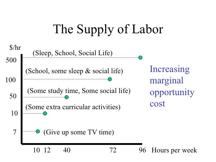
If you were offered a job doing data entry this semester and could work as many hours as you wanted, how many hours per week would you work at minimum wage? The answer to this would be based on your opportunity cost. What would you have to give up – social time, study time, or another job?
An individual may be willing to work a few hours at a low wage since the value of what they are sacrificing is relatively low. As the wage rate rises, individuals are typically willing to work more hours since the marginal benefit becomes greater than or equal to the marginal cost of what has to be sacrificed. At some point, many students would choose to drop out of school for the semester since the marginal benefit is greater than the marginal cost. Many stars and celebrities never attend college or drop out since the income that they would be foregoing at that time in their lives, exceeds the increase in their earnings potential of attending school.
The climate and soils of Idaho allow it to grow some of the best potatoes in the world. At a given price, farmers are willing to supply a certain number of potatoes to the market. Since farmers have already used their land best suited for potato production they have to use land that is less suitable to potato production if they want to grow more potatoes. Since this land is less suited for potato production, yields are lower and the cost per hundredweight of potatoes is greater. As the price of potatoes increases, farmers are able to justify growing more potatoes even though the marginal cost is greater.
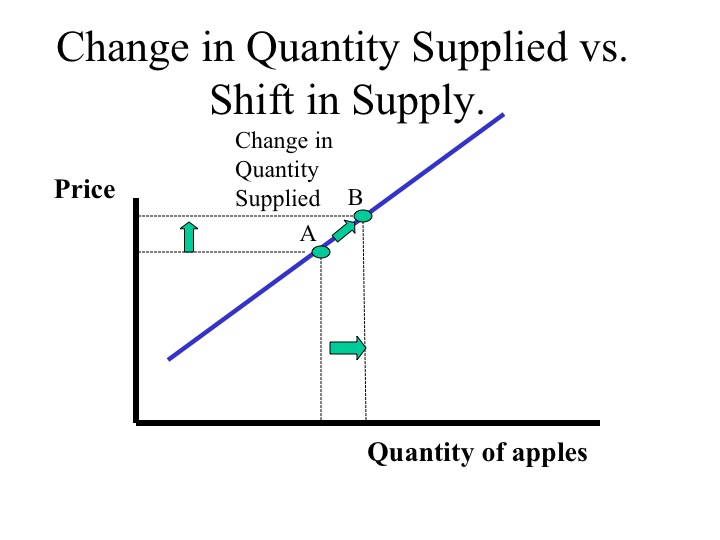
Similar to the demand curve, a movement along the supply curve from point A to point B is called a change in the quantity supplied. Changes along the supply curve are caused by a change in the price of the good. As the price of the apples increases, producers are willing to supply more apples.
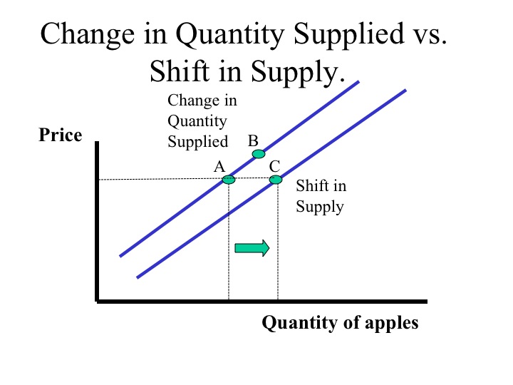
A shift in the supply curve (for example from A to C) is caused by a factor other than the price of the good and results in a different quantity supplied at each price.
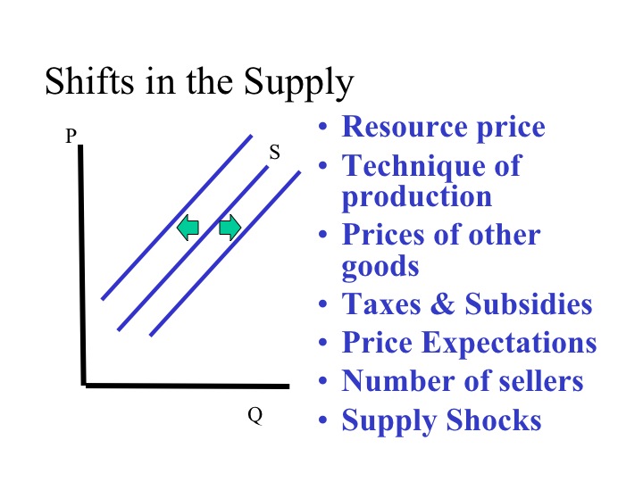
Factors that Shift the Supply Curve
The factors listed below will shift the supply curve either out or in.
1. Resource price
If the price of crude oil (a resource or input into gasoline production) increases, the quantity supplied of gasoline at each price would decline, shifting the supply curve to the left.
2. Technique of production
If a new method or technique of production is developed, the cost of producing each good declines and producers are willing to supply more at each price - shifting the supply curve to the right.
3. Prices of other goods
If the price of wheat increases relative to the price of other crops that could be grown on the same land, such as potatoes or corn, then producers will want to grow more wheat, ceteris paribus. By increasing the resources devoted to growing wheat, the supply of other crops will decline. Goods that are produced using similar resources are substitutes in production.
Complements in production are goods that are jointly produced. Beef cows provide not only steaks and hamburger but also leather that is used to make belts and shoes. An increase in the price of steaks will cause an increase in the quantity supplied of steaks and will also cause an increase (or shift right) in the supply of leather which is a complement in production.
4. Taxes & Subsidies
Taxes and subsidies impact the profitability of producing a good. If businesses have to pay more taxes, the supply curve would shift to the left. On the other hand, if businesses received a subsidy for producing a good, they would be willing to supply more of the good, thus shifting the supply curve to the right.
5. Price Expectations
Expectations about the future price will shift the supply. If sellers anticipate that home values will decrease in the future, they may choose to put their house on the market today before the price falls. Unfortunately, these expectations often become self-fulfilling prophecies, since if many people think values are going down and put their house on the market today, the increase in supply leads to a lower price.
6. Number of sellers
If more companies start to make motorcycles, the supply of motorcycles would increase. If a motorcycle company goes out of business, the supply of motorcycles would decline, shifting the supply curve to the left.
7. Supply Shocks
The last factor is often out of the hands of the producer. Natural disasters such as earthquakes, hurricanes, and floods impact both the production and distribution of goods. While supply shocks are typically negative, there can be beneficial supply shocks with rains coming at the ideal times in a growing season.
To recap, changes in the price of a good will result in movements along the supply curve called changes in quantity supplied. A change in any of the other factors we've discussed (and listed above), will shift the supply curve either right or left. The resulting movements are called changes in supply.
Practice
Identify how each factor will shift the supply curve: right, left, or move along.
| Market | Change |
| 1. Computers | Price of memory chips decreases. |
| 2. Airline Tickets | Government imposes a new jet fuel tax. |
| 3. Milk | Demand for milk increases. |
| 4. Homes | Potential sellers expect home prices to decline in six months. |
| 5. Cars | A new engine design reduces the cost of producing cars. |
| 6. Corn | The price of wheat (a substitute in production increases in price). |
| 7. Oranges | A freeze in Florida kills 25% of the orange crop. |
1. S-Right 2. S-Left 3. Along-Greater Q 4. S-Right 5. S-Right 6. S-Left 7. S-Left
Section 03: Equilibrium
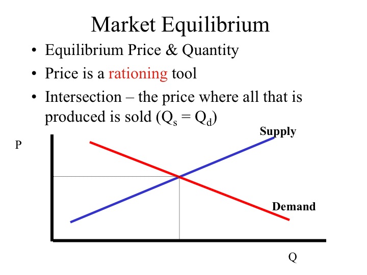
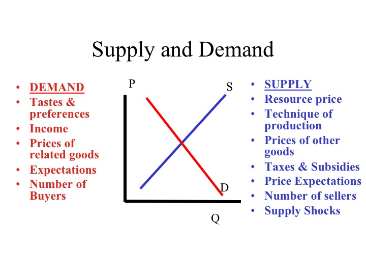
A market brings together those who are willing and able to supply the good and those who are willing and able to purchase the good. In a competitive market, where there are many buyers and sellers, the price of the good serves as a rationing mechanism. Since the demand curve shows the quantity demanded at each price and the supply curve shows the quantity supplied, the point at which the supply curve and demand curve intersect is the point at where the quantity supplied equals the quantity demanded. This is call the market equilibrium.
Consumer Surplus and Producer Surplus
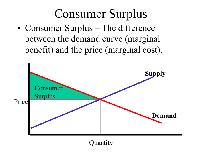
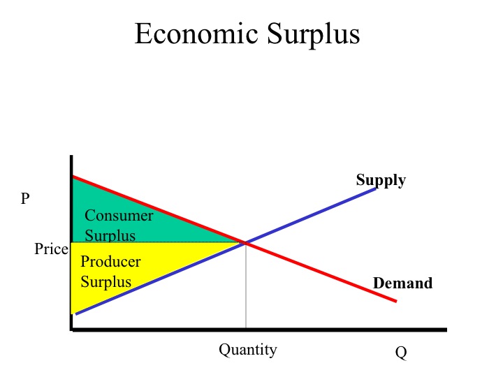
At the last unit purchased, the price the consumer pays (their marginal cost) is equal to what they were willing to pay (the marginal benefit). The previous units purchased actually cost less than what consumers were willing to pay. This difference between the demand curve, i.e., what consumers were willing to pay and the price, i.e., what consumers had to pay, is known as the consumer surplus.
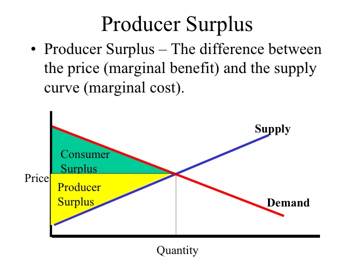
The marginal cost of producing a good is represented by the supply curve. The price received by the sale of the good would be the marginal benefit to the producer, so the difference between the price and the supply curve is the producer surplus, the additional return to producers above what they would require to produce that quantity of goods.
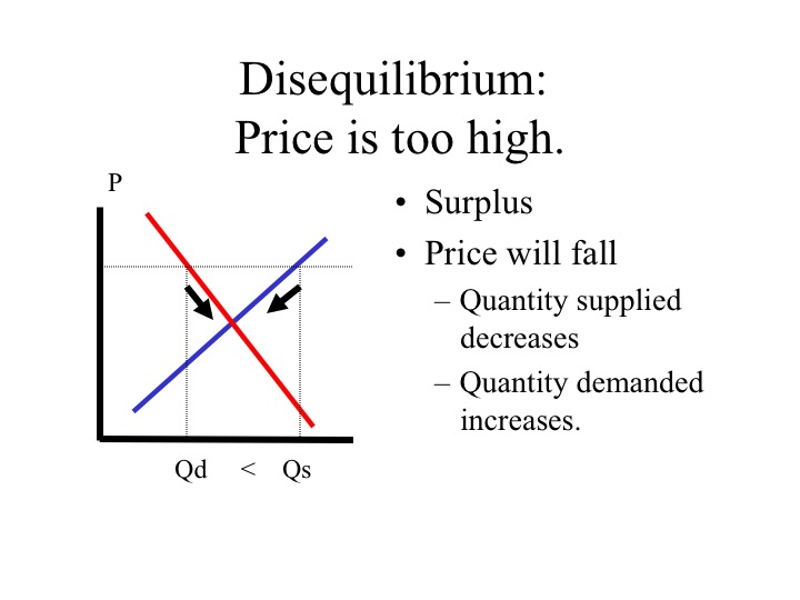
If the market price is above the equilibrium, the quantity supplied will be greater than the quantity demanded. The resulting surplus in the market will lead producers to cut back on production and lower the price. As the price falls, the quantity demanded increases since consumers are willing to buy more of the product at the lower price. In a competitive market, this process continues till the market reaches equilibrium. While a market may not be in equilibrium, the forces in the market move the market towards equilibrium.
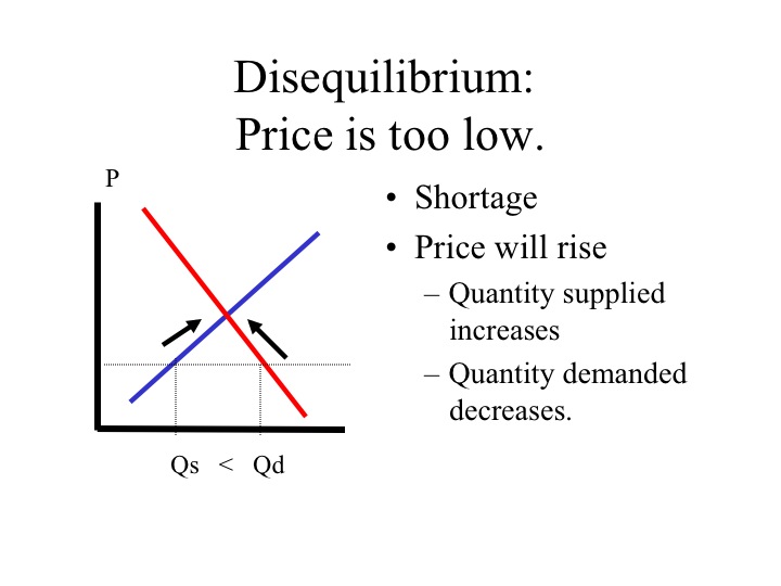
If the market price is too low, consumers are not able to purchase the amount of the product they desire at that price. As a result of this shortage, consumers will offer a higher price for the product. As the price increases, producers are willing to supply more of the good, but the quantity demanded by consumers will decrease. Forces in the market will continue to drive the price up until the quantity supplied equals the quantity demanded.
The factors of supply and demand determine the equilibrium price and quantity. As these factors shift, the equilibrium price and quantity will also change.
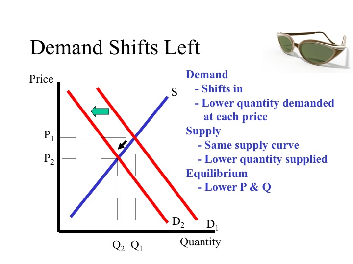
If the demand decreases, for example a particular style of sunglasses becomes less popular, i.e., a change a tastes and preferences, the quantity demanded at each price has decreased. At the current price there is now a surplus in the market and pressure for the price to decrease. The new equilibrium will be at a lower price and lower quantity. Note that the supply curve does not shift but a lower quantity is supplied due to a decrease in the price.
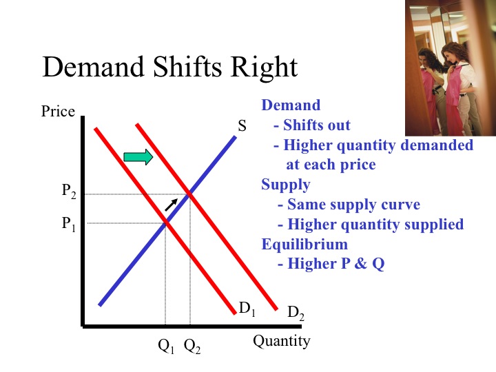
If the demand curve shifts right, there is a greater quantity demanded at each price, the newly created shortage at the original price will drive the market to a higher equilibrium price and quantity. As the demand curve shifts the change in the equilibrium price and quantity will be in the same direction, i.e., both will increase.
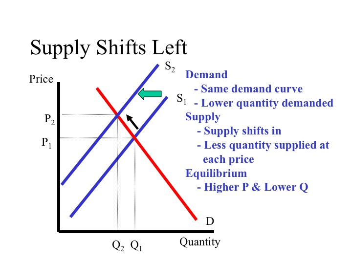
If the supply curve shifts left, say due to an increase in the price of the resources used to make the product, there is a lower quantity supplied at each price. The result will be an increase in the market equilibrium price but a decrease in the market equilibrium quantity. The increase in price, causes a movement along the demand curve to a lower equilibrium quantity demanded.
A rightward shift in the supply curve, say from a new production technology, leads to a lower equilibrium price and a greater quantity. Note that as the supply curve shifts, the change in the equilibrium price and quantity will be in opposite directions.
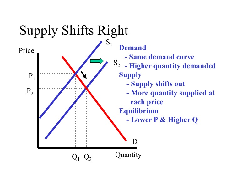
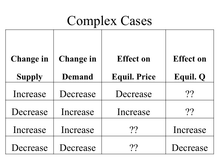
When demand and supply are changing at the same time, the analysis becomes more complex. In such cases, we are still able to say whether one of the two variables (equilibrium price or quantity) will increase or decrease, but we may not be able to say how both will change. When the shifts in demand and supply are driving price or quantity in opposite directions, we are unable to say how one of the two will change without further information.
We are able to find the market equilibrium by analyzing a schedule or table, by graphing the data or algebraically.
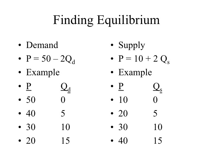
Even without graphing the curves, we are able to analyze the table and see that at a price of $30 the quantity demanded equals the quantity supplied. This is clearly the equilibrium point.
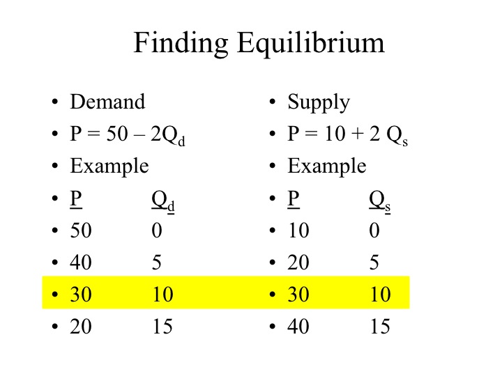
If we graph the curves, we find that at price of 30 dollars, the quantity supplied would be 10 and the quantity demanded would be 10, that is, where the supply and demand curves intersect.
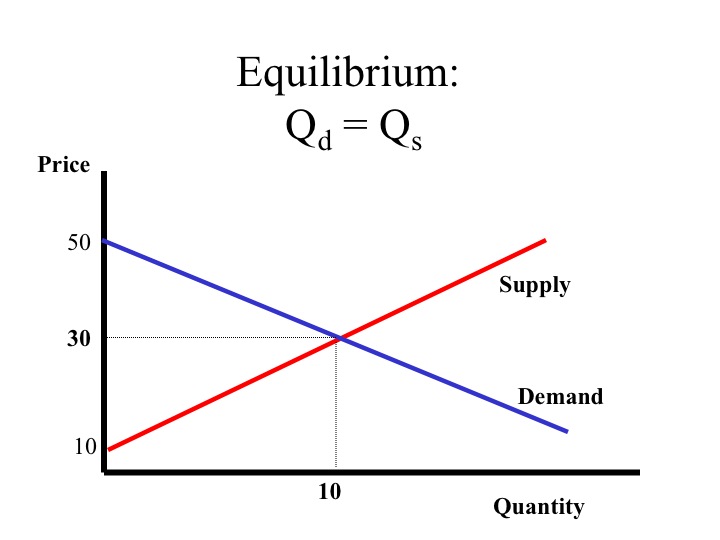
The data can also be represented by equations.
P = 50 – 2Qd and P = 10 + 2 Qs
Solving the equations algebraically will also enable us to find the point where the quantity supplied equals the quantity demanded and the price where that will be true. We do this by setting the two equations equal to each other and solving. The steps for doing this are illustrated below.
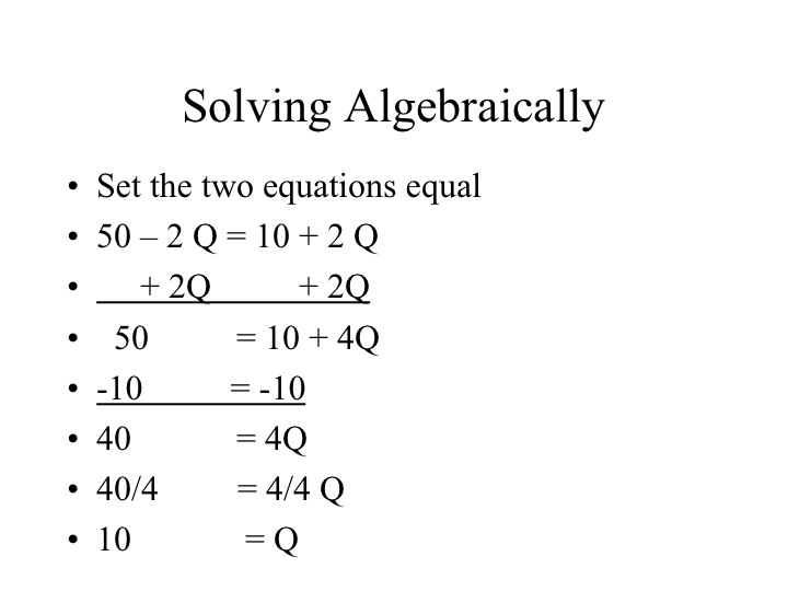
Our first step is to get the Qs together, by adding 2Q to both sides. On the left hand side, the negative 2Q plus 2Q cancel each other out, and on the right side 2 Q plus 2Q gives us 4Q. Our next step is to get the Q by itself. We can subtract 10 from both sides and are left with 40 = 4Q. The last step is to divide both sides by 4, which leaves us with an equilibrium Quantity of 10.
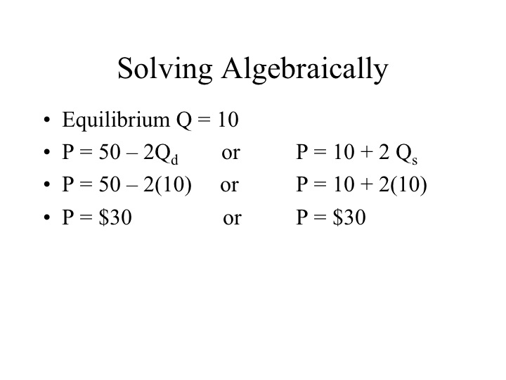
Given an equilibrium quantity of 10, we can plug this value into either the equation we have for supply or demand and find the equilibrium price of $30. Either graphically or algebraically, we end up with the same answer.
Section 04: Market Intervention
If a competitive market is free of intervention, market forces will always drive the price and quantity towards the equilibrium. However, there are times when government feels a need to intervene in the market and prevent it from reaching equilibrium. While often done with good intentions, this intervention often brings about undesirable secondary effects. Market intervention often comes as either a price floor or a price ceiling.
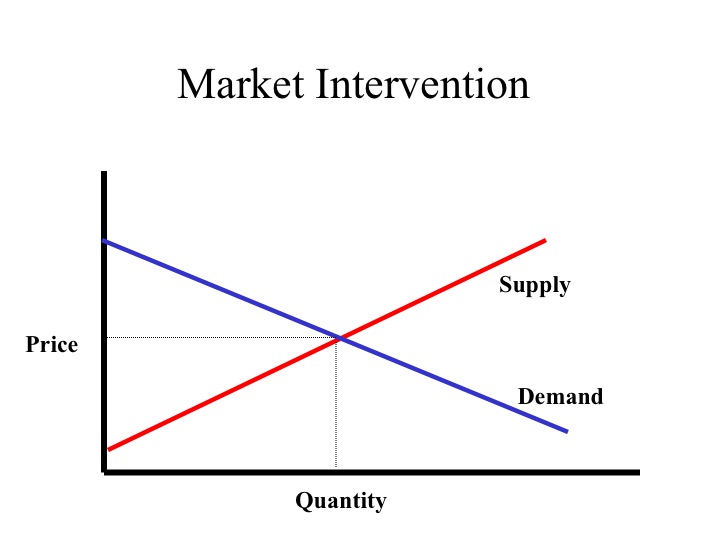
A price floor sets a minimum price for which the good may be sold. Price floors are designed to benefit the producers providing them a price greater than the original market equilibrium. To be effective, a price floor would need to be above the market equilibrium. At a price above the market equilibrium the quantity supplied will exceed the quantity demanded resulting in a surplus in the market.
For example, the government imposed price floors for certain agricultural commodities, such as wheat and corn. At a price floor, greater than the market equilibrium price, producers increase the quantity supplied of the good. However, consumers now face a higher price and reduce the quantity demanded. The result of the price floor is a surplus in the market.
Since producers are unable to sell all of their product at the imposed price floor, they have an incentive to lower the price but cannot. To maintain the price floor, governments are often forced to step in and purchase the excess product, which adds an additional costs to the consumers who are also taxpayers. Thus the consumers suffer from both higher prices but also higher taxes to dispose of the product.
The decision to intervene in the market is a normative decision of policy makers, is the benefit to those receiving a higher wage greater than the added cost to society? Is the benefit of having excess food production greater than the additional costs that are incurred due to the market intervention?
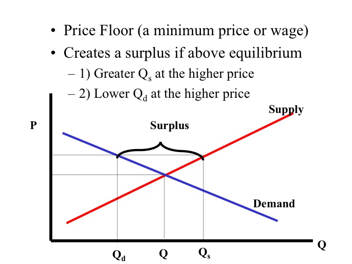
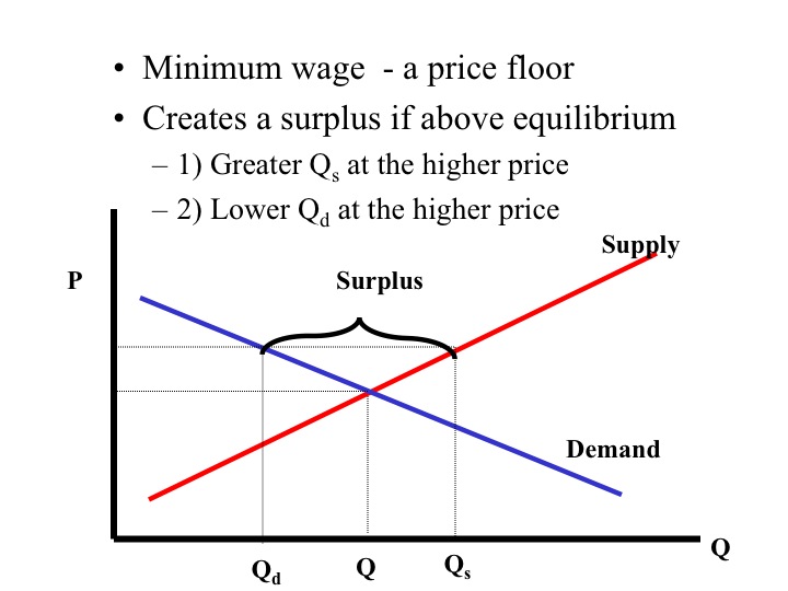
Another example of a price floor is a minimum wage. In the labor market, the workers supply the labor and the businesses demand the labor. If a minimum wage is implemented that is above the market equilibrium, some of the individuals who were not willing to work at the original market equilibrium wage are now willing to work at the higher wage, i.e., there is an increase in the quantity of labor supplied. Businesses must now pay their workers more and consequently reduce the quantity of labor demanded. The result is a surplus of labor available at the minimum wage. Due to the government imposed price floor, price is no longer able to serve as the rationing device and individuals who are willing and able to work at or below the going minimum wage may not be able to find employment.
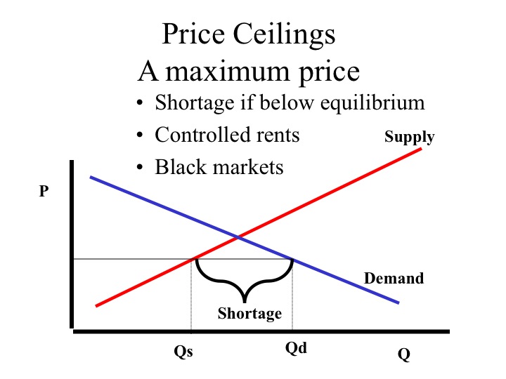
Price ceilings are intended to benefit the consumer and set a maximum price for which the product may be sold. To be effective, the ceiling price must be below the market equilibrium. Some large metropolitan areas control the price that can be charged for apartment rent. The result is that more individuals want to rent apartments given the lower price, but apartment owners are not willing to supply as many apartments to the market (i.e., a lower quantity supplied). In many cases when price ceilings are implemented, black markets or illegal markets develop that facilitate trade at a price above the set government maximum price.
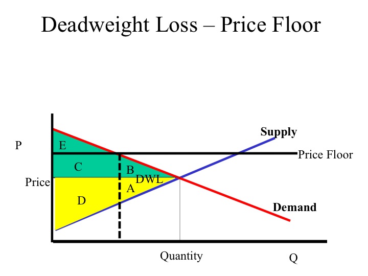
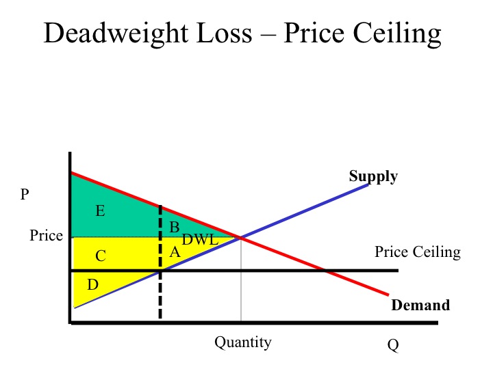
In a competitive market, the economic surplus which is the combined area of the consumer and producer surplus is maximized.
When a price floor is imposed, there is a loss in the economic surplus (Area A and B) known as deadweight loss. Since consumer surplus is the area below the demand curve and above the price, with the price floor the area of consumer surplus is reduced from areas B, C, and E to only area E. Producer surplus which is below the price and above the supply or marginal cost curve changes from area A and D to D and C.
A price ceiling also creates a deadweight loss of area A and B. The consumer surplus area changes from areas E and B to E and C and the producer surplus area is reduced from A, C, and D to only D.
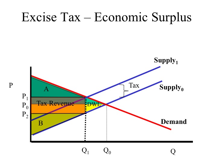
Another government market intervention is the imposition of a tax or subsidy. An excise tax is a tax levied on the production or consumption of a product. To consumers, the tax increases the price of the good purchased moving them along the demand curve to a lower quantity demanded. The vertical distance between the original and new supply curve is the amount of the tax. Due to the tax, the new equilibrium price (P1) is higher and the equilibrium quantity (Q1) is lower. While the consumer is now paying price (P1) the producer only receives price (P2) after paying the tax.
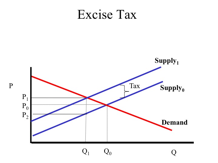
Due to the tax, the area of consumer surplus is reduced to area A and producer surplus is reduced to area B. The tax revenue is equal to the tax per unit multiplied by the units sold. The areas of consumer and producer surplus that were to the right of Q1 are lost and make up the deadweight loss.
