Fiscal Policy
Discretionary fiscal policy refers to the deliberate manipulation of taxes and government spending by Congress to alter real output and employment (thus impacting economic growth) and to control inflation. The word “discretionary” means that the policy changes are at the discretion or option of the Federal government. When fiscal policy is used to try to increase output and reduce unemployment, it is called expansionary; when fiscal policy is used to try to lower inflation, it is referred to as contractionary.
Section 01: Expansionary Fiscal Policy
Fiscal Policy can be used to combat a recession. Expansionary fiscal policy is most often used during periods of high cyclical unemployment, when policy makers feel that stimulating economic growth and increasing real output can be done with either no impact on price levels in the economy or with minimal inflation at an acceptable level. Which fiscal policies would be recommended during a recession? There are two policies that would be expansionary (think of shifting the Aggregate Demand curve to the right): the first would be a decrease in taxes and the second would be an increase in government spending. Let’s look at the impact of each.
A decrease in taxes raises consumption by the MPC times the decrease in taxes and then will shift the AD to the right by a multiple of the change in consumption. It will be helpful to walk through this process and look at it graphically with an example. Let’s say that the government decides to reduce taxes by one million dollars. When consumers are informed that their taxes are going down by one million dollars, they will find that they now have one million dollars that they thought they were going to have to pay in taxes that they are actually going to be allowed to keep. In many ways, this will seem to them like a one million dollar increase in income. How much of the one million dollars will they actually spend? This depends on the MPC. For example, if the MPC is equal to .8, consumers will spend $800,000 when their taxes are reduced by one million dollars. What will they do with the other $200,000? They will save it, because if their MPC is equal to .8, their MPS is equal to .2.
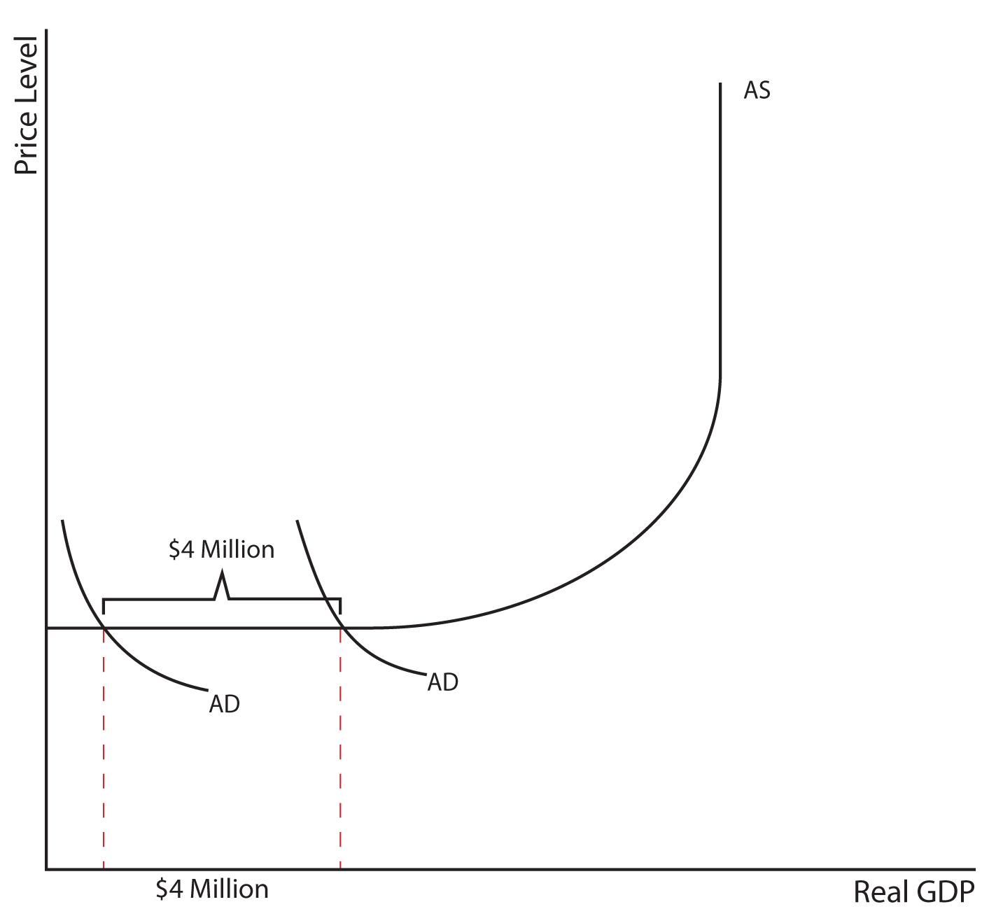
The increase in Consumption of $800,000 is going to shift the AD to the right, but by how much? With an MPC of .8, the expenditures multiplier is equal to 5 and the AD curve will be shifted by $4,000,000. Since expansionary policy is used to combat a recession, we will assume that the AD intersects the AS curve in either the Keynesian Range or in the Intermediate Range (i.e., we would not use expansionary policy if the AD curve intersects the AS curve in the Classical Range). Let’s look at the impact on real output and the price level of a $4 million shift in the AD curve in each of the two possible ranges mentioned above.
If the AD curve intersects the AS in the Keynesian Range a $4 million shift in AD will result in no changes in the price level and a $4 million increase in real output. This result corresponds to the result that we would have found in the Aggregate Expenditures lesson that we had previously.
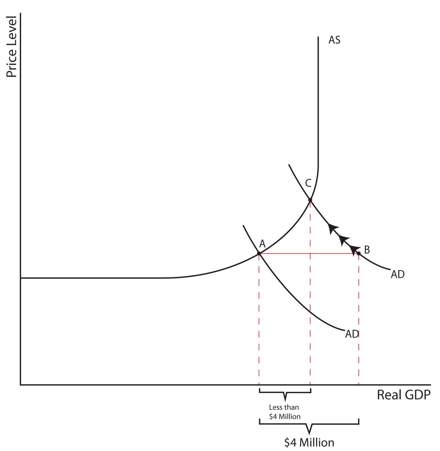
If the AD curve intersects the AS curve in the intermediate range the same $4 million shift in AD will cause prices to rise which will dampen the increase in real output. As prices go up, components of the AD (C, I, and NX) curve will react to those higher prices, which will cause spending in those area to decrease. As shown below, the shift in AD can be expressed as the movement from point A to point B, but the eventual impact on real output when the AD is in the Intermediate Range of AS is shown by the shift from point A to point C. The movement upward along the AD curve from point B to point C illustrates the impact on C, I, and NX of increases in the price level. In brief, just remember the Real Balances, Interest Rate, and Foreign Purchases Effects from a previous lesson.
In the case of both the AD intersecting AS in the Keynesian Range and in the Intermediate Range, expansionary fiscal policy reduces unemployment because it increases real GDP. In the case where AD is in the intermediate range the increase in government spending or reduction in taxes will cause inflation. While this discussion of expansionary fiscal policy has been in terms of an increase in government spending OR a decrease in taxes, it should go without saying that a combination of these two policies is also expansionary.
Section 02: Contractionary Fiscal Policy
Fiscal Policy can be used to combat excessive demand-pull inflation as well. Contractionary fiscal policy is most often used during periods of high inflation when policy makers believe contracting the economy (and thereby reducing inflation) is possible with either no impact on or minimal reductions in real output, causing small increases in unemployment that would be considered acceptable. Which fiscal policies would be recommended during a period of high inflation? There are two policies that would be contractionary (think of shifting the Aggregate Demand curve to the left): the first would be a decrease in government spending and the second would be an increase in taxes. Since contractionary policy is used to combat inflation and since inflation is not an issue in the Keynesian range of the AS curve, we will assume that contractionary policy is only used when the AD intersects the AS in the latter’s classical range or intermediate range.
Consider first the impact of contractionary fiscal policy when the AD intersects the AS curve in its classical range. A decrease in government spending or an increase in taxes reduces AD by a multiple of the dollar amount of the fiscal policy and shifts the AD curve to the left. In the classical range, the reduction in AD lowers the price sufficiently to stimulate C, I, and NX to the point that output stays at the full-employment level. The result is that the price level in the economy rises but output and employment stay the same.
In the case where the AD curve intersects the AS curve in the intermediate range, the contractionary fiscal policy reduces prices—but not so much that the resulting increases in C, I, and NX are not enough to keep output at the full-employment level. Reductions in the price level are accompanied by reductions in real output and employment, possibly causing unemployment.
Return to the course in I-Learn and complete the activity that corresponds with this material.
Section 03: Financing the Deficit
The method used to finance a deficit brought about by expansionary fiscal policy will influence the extent of the expansionary effect. Let’s look at two possible ways of financing the deficit. The government can finance a deficit the same way a household would: borrowing. In this case, the government competes with private borrowing for funds. The market for loanable funds has supply and demand. If the government tries to borrow money from the public (say, through issuing savings bonds), the money lent to the government is no longer available to supply the private market, and the supply of loanable funds shifts to the left. This drives up interest rates, which will “crowd out” private investment. As private investment falls, the AD shifts back to the left, thus off-setting the expansionary effects of the increase in government spending.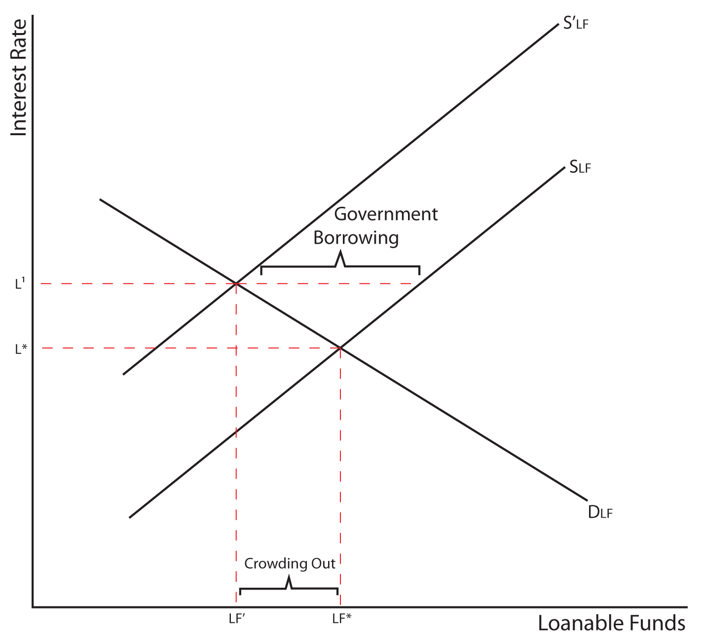
In the second case, the Federal Reserve essentially loans directly to the government by buying bonds which does not impact the private loanable funds market, and does not influence interest rates. Since there is no impact on private investment, the expansionary effect is greater than by borrowing because there is no crowding out effect. Since this method of financing the deficit is closely tied to monetary policy, not fiscal policy, we will discuss it in more detail later.
The Supply Side of Fiscal Policy
Until now, we have focused on the demand side of fiscal policy. There is an important way in which fiscal policies can influence the potential output of the economy through the supply side as well. On the government spending side, fiscal policies geared toward building infrastructure such as roads, bridges, airports, etc., can impact the future productive capacity of the economy and stimulate long-run economic growth. In short, certain types of government spending can influence the ability of the AS curve to shift to the right over time. On the tax side of fiscal policy, we can influence the long-run growth of the economy by the work incentives that our tax codes either stimulate or reduce in families and the productive incentives that our tax codes can either stimulate or reduce in firms.
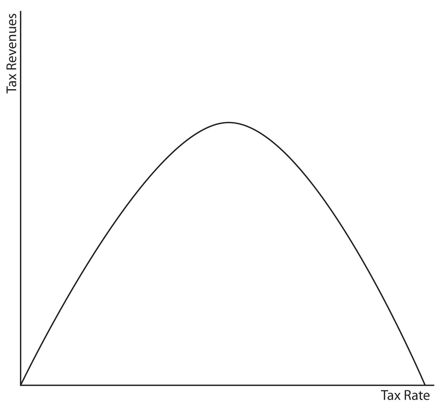
Economist Arthur Laffer was an early proponent of the idea that if tax rates are too high, it can actually give individuals an incentive to work less and thereby lower tax revenues. The graph below has come to be known as the Laffer Curve and illustrates this point. Laffer suggested in the 1970s that we were on the downward sloping side of the Laffer Curve and that if the United States were to lower tax rates we could actually increase tax revenues. While there is some debate as to the validity of Laffer’s argument, it is interesting to note that when President Ronald Reagan followed Laffer’s guidance in this matter and lowered tax rates following his election, tax revenues increased each and every year of his presidency.
Which is Better—Government Spending or Taxes?
“Liberal” economists tend to favor higher government spending during a recession (expansionary policy) and higher taxes during inflationary times (contractionary policy). Both of these policies envision a larger role for the government in the economy.
“Conservative” economists tend to favor lower taxes during a recession (expansionary policy) and lower government spending during inflationary times (contractionary policy). Both of these policies envision a smaller role for the government in the economy.
As would be the case for most groups in the country, there is no consensus among economists about which policies are preferable.