Aggregate Demand and Aggregate Supply

Section 01: Aggregate Demand

As discussed in the previous lesson, the aggregate expenditures model is a useful tool in determining the equilibrium level of output in the economy. It does have a significant flaw, however: the aggregate expenditures model does not take into account the impact of the price level on aggregate output. The Aggregate Demand Curve (AD) represents, in that sense, an even more appropriate model of aggregate output, because it shows the various amounts of goods and services which domestic consumers (C), businesses (I), the government (G), and foreign buyers (NX) collectively will desire at each possible price level. Let’s begin by showing the relationship between the aggregate expenditures model and the AD curve.

In the graph below, we show the standard aggregate expenditures curve at three different price levels. When prices are high (P1), Consumption is low; as prices fall to P2 and P3, Consumption rises. As the Consumption function shifts upward due to the falling prices, the equilibrium level of GDP goes up from GDP1 to GDP3. This is depicted in the AD framework as a downward sloping AD curve.

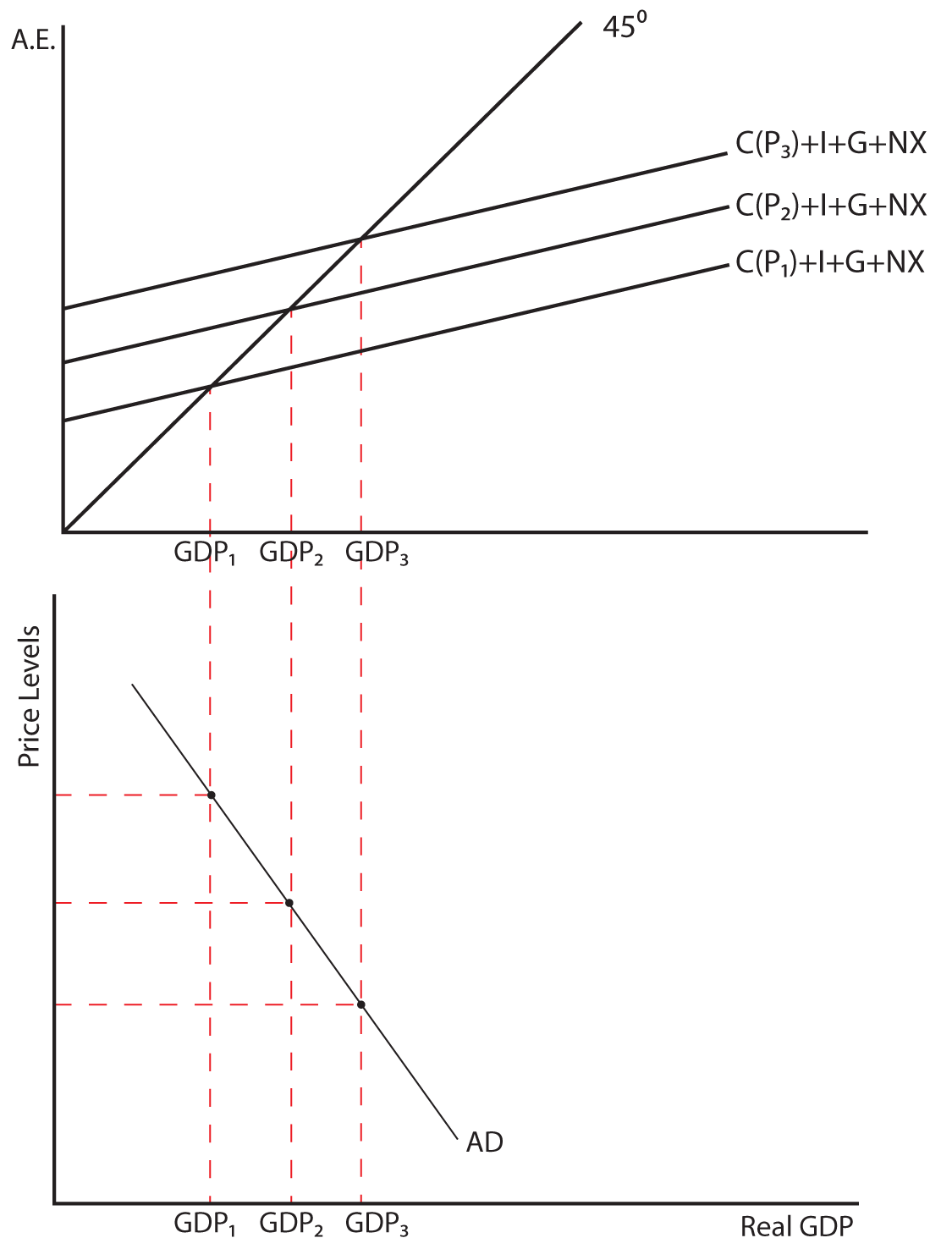
Why does it make sense for the AD curve to slope downward and to the right? We will suggest three different rationales for the downward sloped curve: the real balances effect, the interest rate effect, and the foreign purchases effect.

The Real Balances Effect

“Real balances” refers to the purchase power of a given amount of money in circulation. We make the assumption that at any given point in time, there is a fixed amount of money in circulation. At higher price levels, the money in circulation can purchase fewer items. Think of the simple of example of having $1,000 in circulation and the average price of the goods and services in the economy being $10. A total of 100 items could be purchased under these conditions. If the average price level were to rise to $20 per item, then the $1,000 in circulation would only allow us to purchase 50 items. At higher prices, the money in circulation will spread over fewer goods. When prices fall, the purchasing power of the money in circulation goes up, and people can buy more goods and services. This relationship between prices and the amount of goods and services that can be purchased with a given money supply is called the real balances effect. It justifies our depiction of the AD curve as a downward sloping curve.

The Interest Rate Effect

The interest rate effect explains impact that the price level has on interest rates, and thus on certain components of AD. When the price level goes up, people need more money to transact their daily purchases. Therefore, higher prices lead to an increase in the demand for money. With a fixed amount of money in circulation, increasing the demand for money will cause the interest rate to go up. Think of how you would behave if you were running a bank and the demand for money increased. You would try to encourage additional people to deposit money into the bank, and at the same time discourage people from coming into the bank to demand money. The way to do both simultaneously would be to increase the interest rate. As interest rates go up, investment demand and certain interest-rate sensitive consumption purchases will fall. Thus, increases in the price lead to increases the interest rate, which reduces the demand for both Consumption and Investment, and thus real output. The interest rate effect is therefore an additional justification for the downward sloping AD curve.

The Foreign Purchases Effect

Domestic prices also have an impact on Net Exports (NX) through what is called the foreign purchases effect. When US prices rise relative to world prices, foreigners buy fewer US goods and Americans buy more foreign goods, so NX fall. Since NX are part of AD, this contributes to an inverse relationship between the price level and the demand for our real domestic output. The opposite is also true. The foreign purchases effect contributes to our argument for why the AD is downward sloping.

Anything that changes the price level triggers these three effects and is represented by movement along a given AD curve. There are other factors that influence aggregate demand besides the price level, and these factors are referred to as determinants of AD. When these other factors change, they cause a shift in the entire AD curve and are sometimes called aggregate demand shifters. These aggregate demand shifters include anything that will influence the levels of Consumption, Investment, Government Spending, or Net Exports OTHER THAN changes in the price level. Let’s consider each in turn.

Section 02: Aggregate Demand Shifters

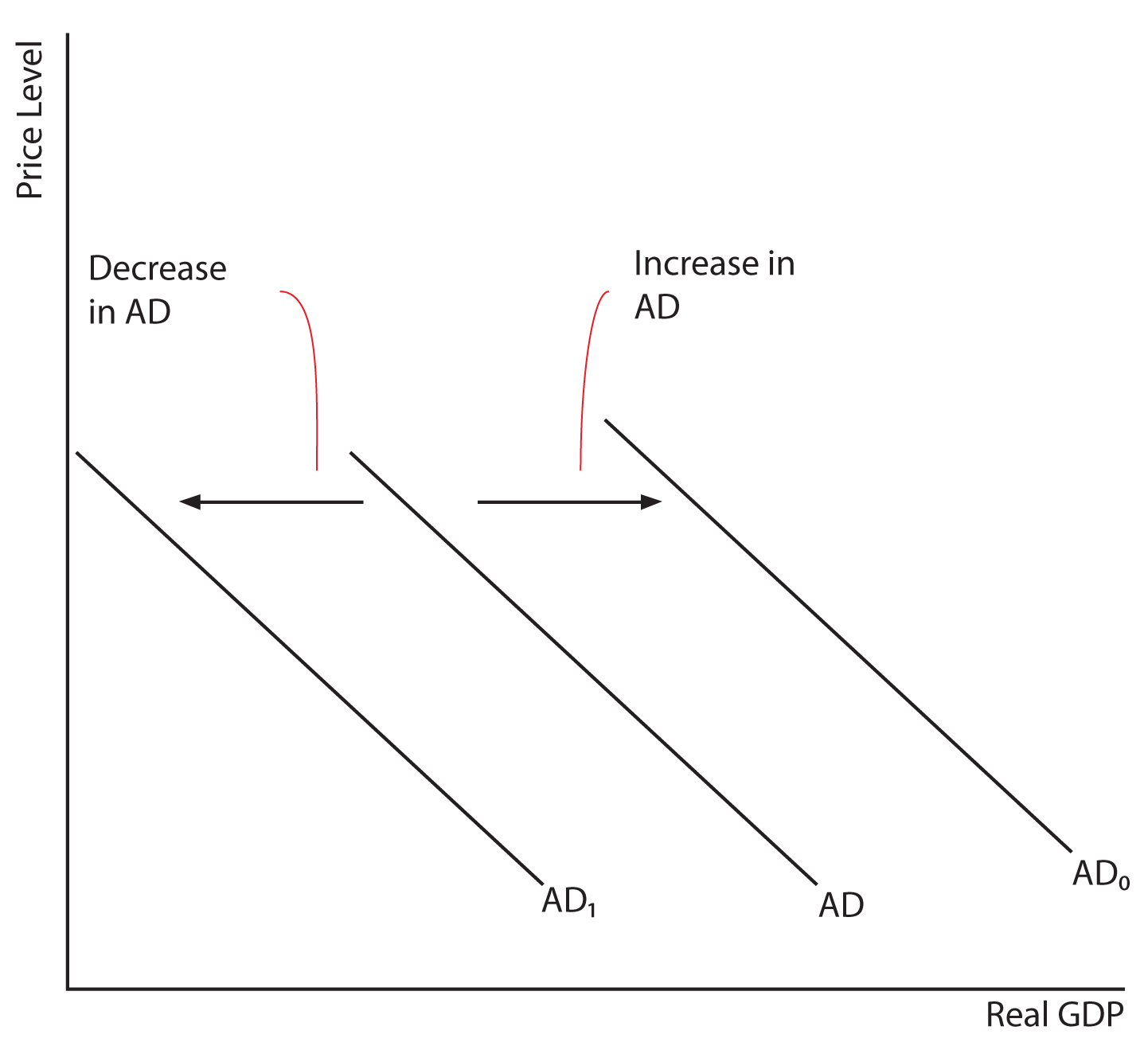
The graph below illustrates what a change in a determinant of aggregate demand will do to the position of the aggregate demand curve. As we consider each of the determinants remember that those factors that cause an increase in AD will shift the curve outward and to the right and those factors that cause a decrease in AD will shift the curve inward and to the left.

Changes in Consumption unrelated to a change in the price

There are several factors that could increase or decrease consumption that are unrelated to changes in the price level. For instance, increases in consumer wealth would increase consumption at each price level and would be illustrated by a rightward shift in AD. Decreases in consumer wealth would have the opposite effect. Increases in consumer indebtedness would decrease consumption and shift the aggregate demand curve to the left, while decreases in indebtedness would have the opposite effect. Increases in taxes will decrease consumption (and shift the AD curve to the left) while decreases in taxes will increase consumption and shift the AD curve to the right. Consumer expectations about the future of the economy can have a strong impact on consumptions. Optimism about the economy will increase consumption and shift the AD curve to the right, while widespread pessimism dampens consumer spending and shifts the AD curve to the left. You can probably think of other factors that will shift the AD curve because they impact consumption independent of the price level.

Changes in Investment unrelated to a change in the price

There are several factors unrelated to changes in the price level that could increase or decrease Investment and thereby shift the AD curve. For instance, any change in the interest rate not brought about by a change in the price level would change the level of investment in the economy, and shift the AD curve. Increases in the interest rate will reduce investment demand; decreases in the interest rate will increase investment demand. Business taxes can be structured to either encourage investment (shifting the AD to the right) or discourage investment (shifting AD to the left). Technological improvements in an industry might make old equipment obsolete and stimulate investment, shifting AD to the right. Finally, like the impact of expectations on consumers, optimism (or pessimism) on the part of business owners can lead to increases (or decreases) in investment activity and shift the AD curve to the right (or left).

Changes in Government Spending unrelated to a change in the price

The political process will sometimes lead to increases or decreases in the level of government spending. Increases in government spending will shift the AD curve to the right; decreases in government spending will shift the AD curve to the left.

Changes in Net Exports unrelated to changes in the price

There are two important factors unrelated to the price level that could increase or decrease the level of Net Exports and thereby shift the AD Curve. The first has to do with changes in national income abroad. As income abroad grows relative to income in the United States, foreigners are able to buy US products more easily and Americans can afford fewer foreign goods. Net exports will go up, shifting the AD curve to the right. If incomes abroad fall relative to income in the US, the AD curve will shift left due to a decrease in net exports. The second factor has to do with exchange rates, or the relative value of our currency to the currency of a trading partner. As an example, let’s say that it takes 90 Japanese Yen to buy one US dollar. If the value of the yen relative to the dollar changes so that it takes 100 Yen to buy one US dollar, this will decrease the amount that Japanese citizens will buy in the US, and increase the amount that US citizens can buy in Japan. This change in the exchange rate will cause net exports to fall and the AD curve to shift to the left. If the Japanese Yen were to appreciate relative to the dollar, net exports would rise and the AD curve would shift to the right.

Return to the course in I-Learn and complete the activity that corresponds with this material.

Section 03: Aggregate Supply

Aggregate Supply (AS) is a curve showing the level of real domestic output available at each possible price level. Typically AS is depicted with an unusual looking graph like the one shown below. There is a specific reason for why the AS has this peculiar shape. The AS curve can be separated into three distinct ranges called the Keynesian Range, the Intermediate Range, and the Classical Range. The various ranges depict three different states in which the economy may find itself. The three states of the economy can all be thought of in relation to what is called the full-employment level of output, labeled Qf in the graph below. We will now discuss each of the three ranges of the AS.

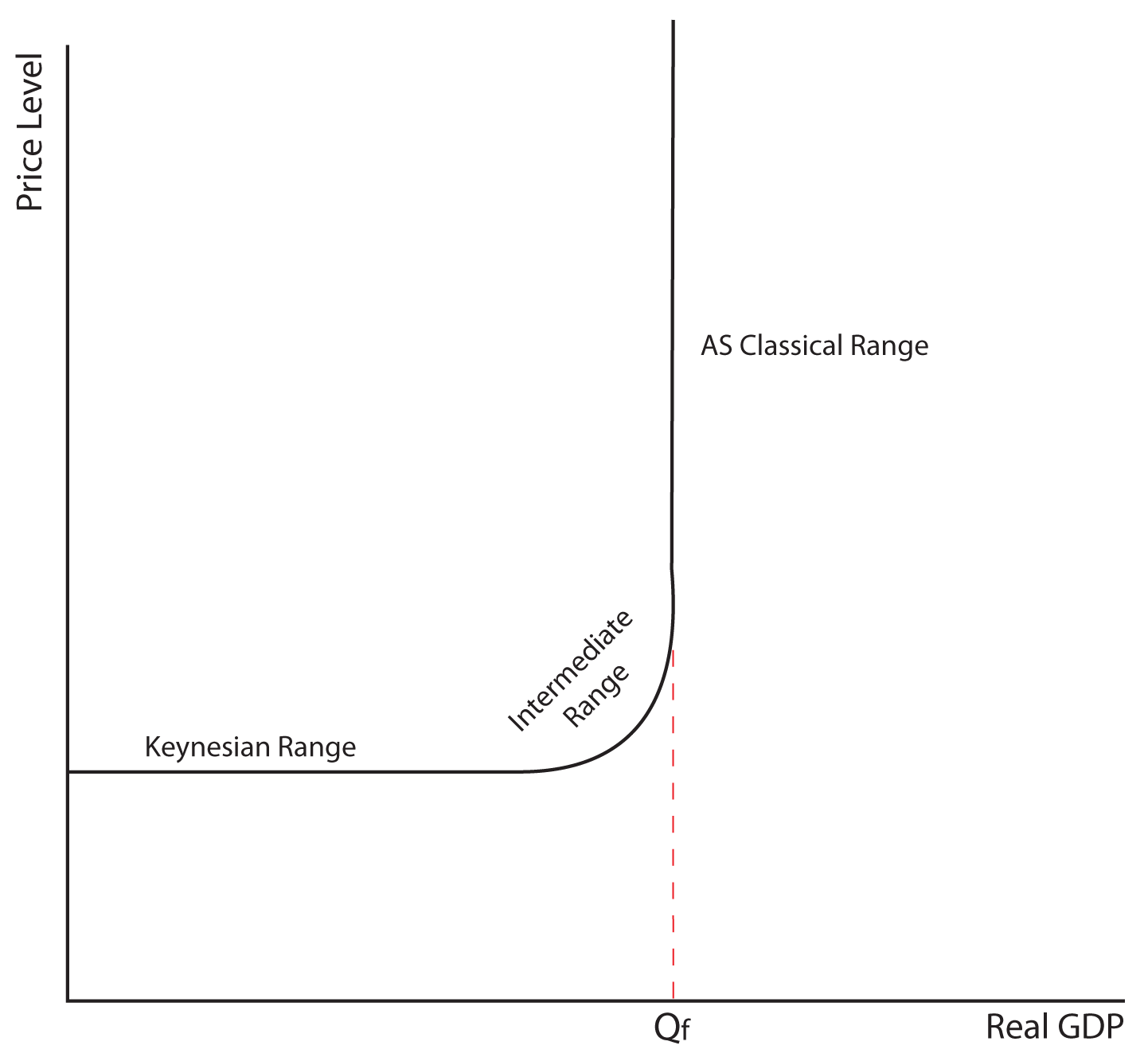
In the Keynesian range of AS, we are at outputs which are substantially below Qf. This horizontal range implies an economy in severe recession or depression. Remember that Keynes wrote his General Theory during the heights of the Great Depression, so the range of AS that is associated with his name corresponds to such an economy. Assume that you were running a factory during a severe recession with high unemployment, and you decided that you would like to increase output. You realize that, to increase output, you are going to have to employ more inputs, primarily more labor—however, a similar argument could be made about high unemployment of any of the other factors of production. You go to the factory door, open it, and find thousands of unemployed workers standing in line, wanting to work at your factory. How much would you have to pay them to get them to go to work for you? Certainly, you would not have to pay them more than the going wage rate in the market, right? Essentially, you could hire as many unemployed resources as you would like without bidding up wages and prices, because of the substantial unemployment. The horizontal or Keynesian AS illustrates the idea of the economy being able to increase real output with no increase in the price level during periods of high unemployment. This range of the AS curve is also sometimes referred to as the Short Run AS curve.

In the Classical Range of AS, we are at or very near the full-employment level of output. This range is named after the Classical Economists who assumed that the economy, in the long run, would always achieve full employment. The Classical AS curve is sometimes called the Long Run AS curve. Assume again that you are running a factory, only this time, the economy is at full-employment. Let’s say again that you want to increase output, and that in order to do so you have to increase the number of workers at your factory. You go to the factory door and open it to find nobody waiting in line. There does not appear to be anyone looking for a job because everyone already has one! In order to hire additional workers, you go to other employers’ workers, and ask them to leave their job to work for you. How much are you going to have to pay these workers to get them to do that? Most likely you will have to pay them more than they are currently making. As you bid up wages in the labor market to attract additional workers, prices in the economy will also rise, because now it costs more to produce your product. That additional cost is passed to the consumer in the form of higher prices, to the extent possible. Attempts to increase output in the Classical Range leads to higher price levels in the economy but what about real GDP? Does it actually increase? Well, your output may go up, but the output of the factory where your new workers used to work will go down, so the overall output in the economy stays the same at Qf.

In the Intermediate Range, we are at output levels that are below full employment, but not so far below as to constitute a deep recession or depression. In this range, increasing output is possible, but only at the expense of rising prices. While that Keynesian Range is a rare short-run occurrence, and the Classical Range is the long-run steady state of the economy, the Intermediate Range is probably where we find ourselves most often in the economy.

Depending on the state of the economy, any attempt to change the output of the economy will move us along a given AS curve. There are factors that influence aggregate supply, illustratable by shifting the AS curve—these factors are referred to as determinants of AS. When these other factors change, they cause a shift in the entire AS curve and are sometimes called aggregate supply shifters. These aggregate supply shifters include Changes in Resource Prices, Changes in Resource Productivity, Business Taxes and Subsidies, and Government Regulations. Let’s consider each in turn.

Section 04: Determinants of Aggregate Supply

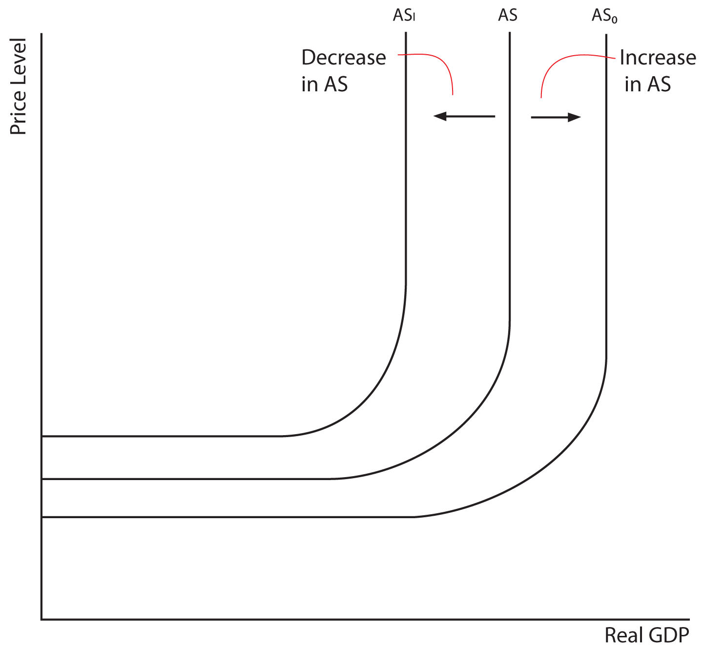
The graph below illustrates what a change in a determinant of aggregate supply will do to the position of the aggregate supply curve. As we consider each of the determinants remember that those factors that cause an increase in AS will shift the curve outward and to the right and those factors that cause a decrease in AS will shift the curve upward and to the left.

Changes in Input Prices

Anything that causes input prices to rise will decrease AS and shift the AS curve to the left. Anything that causes input prices to fall will increase AS and shift the AS curve to the right. For instance, if a particular input into the production process is readily available from domestic suppliers, it will generally be cheaper, holding all else constant (cet. par.). If for no other reason, transportation costs of delivering a domestic resource to a domestic producer will be less than delivering the identical resource from a foreign supplier. That does not even take into account the problems of getting a foreign resource such as duties and tariffs, political or social instability abroad, or other international disruptions. Another factor that can influence input prices would be the market power of the suppliers of the resource. The more competition in the supply of a resource, the cheaper that resource will be, cet. par. If the resource is supplied by a monopolist or a cartel (think OPEC oil), the price of that resource will be higher than if the resource is supplied by a more competitive industry (think corn-produced ethanol).

Changes in Productivity

Independent of its price, anything that makes resources more productive will increase AS and shift the AS curve to the right; anything that makes resources less productive will decrease AS and shift the AS curve to the left. If workers become more productive because of investments in physical or human capital, the economy will be able to produce more and the AS curve will shift to the right. If workers become less productive because of outmoded equipment, insufficient training, or excessive union interference in their workplace, the economy will be less productive, and the AS curve will shift to the left.

Business Taxes and Subsidies

In brief, business taxes increase the cost of production and shift the AS curve to the left; subsidies decrease the cost of production and shift the AS curve to the right.

Government Regulations

Government regulations also influence the costs of production. Increasing government regulations makes it more expensive to produce the nation’s output and shifts the AS curve to the left; reducing government regulations lessens the burden of business and shifts the AS curve to the right.

Return to the course in I-Learn and complete the activity that corresponds with this material.

Section 05: Equilibrium

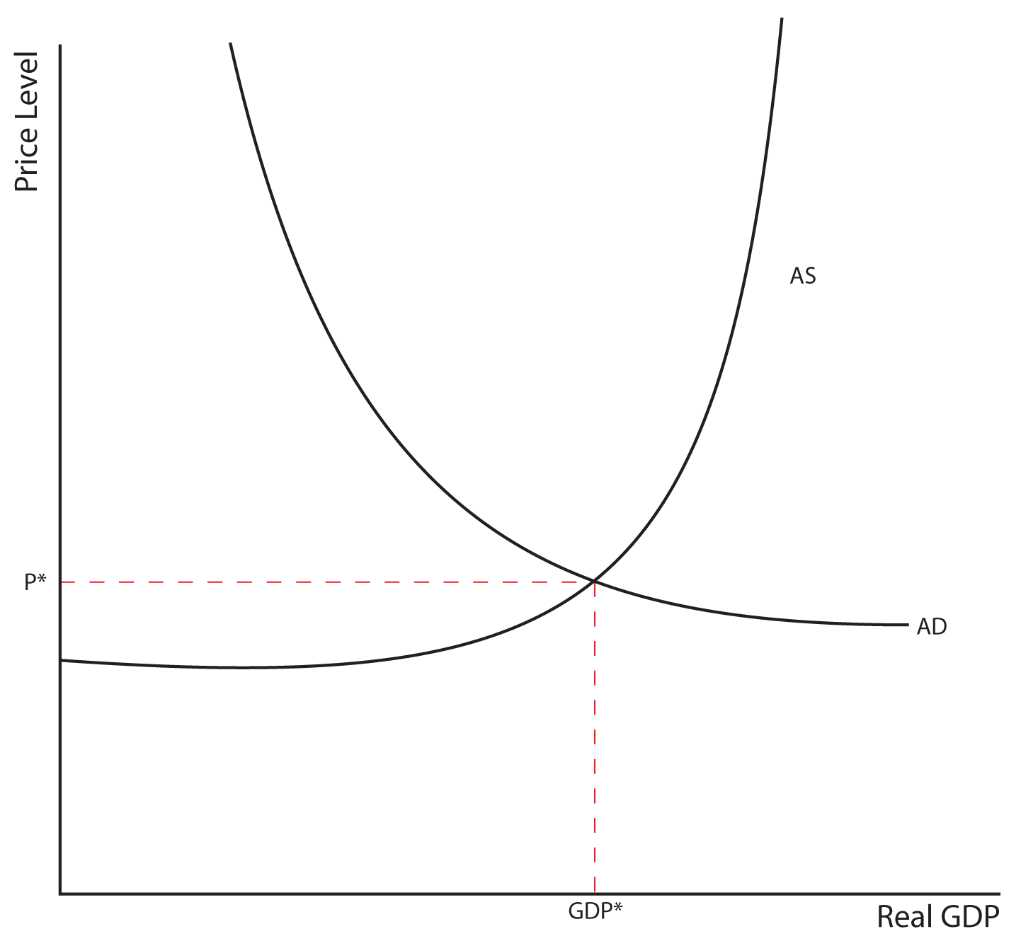
What does the equilibrium between AD and AS determine? The Price Level in the economy and the Real Output (GDP) of the economy. Equilibrium is illustrated below as the intersection between AD and AS.

Section 06: Shifts in the AD Curve

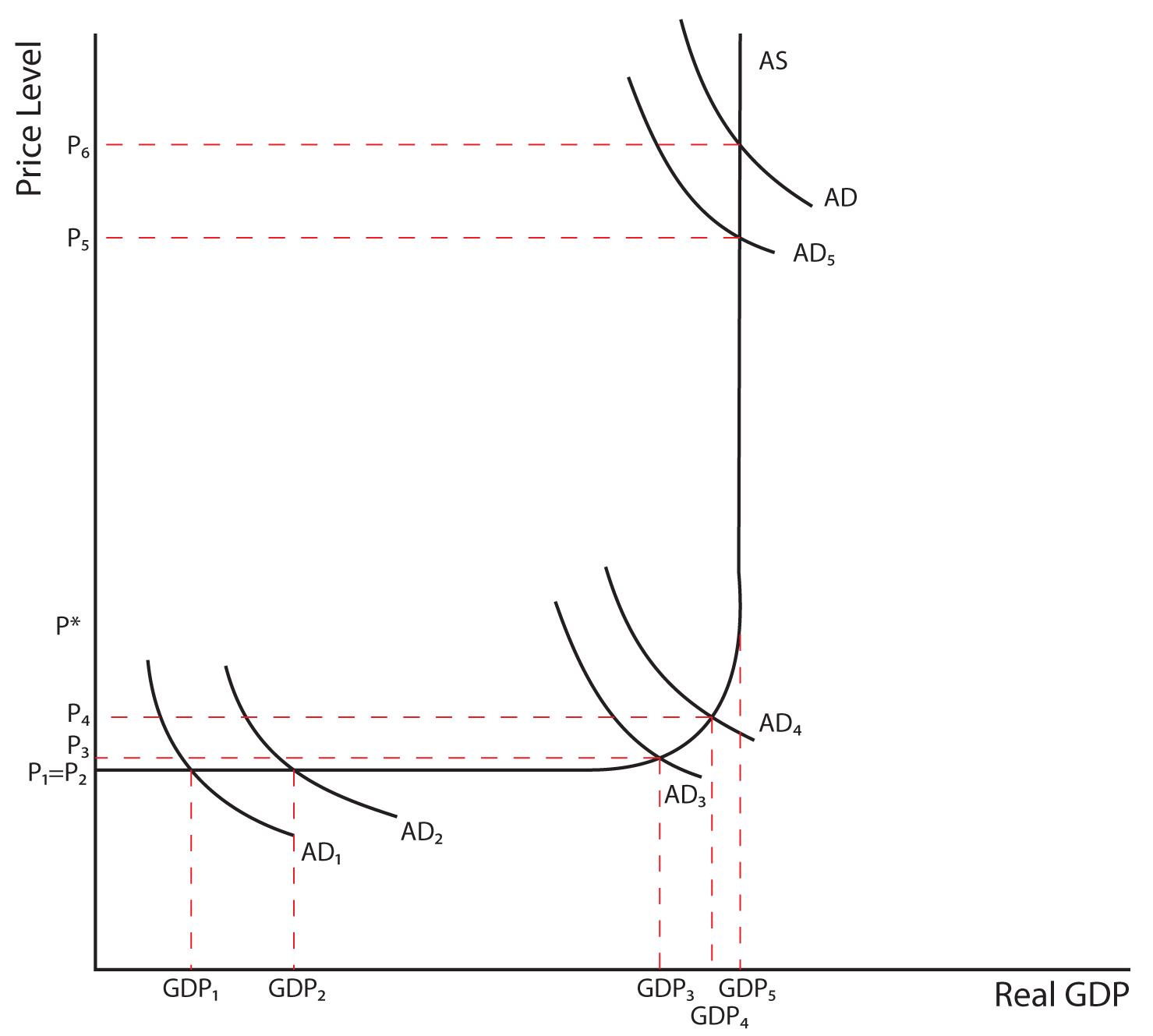
Let’s review all of the possible impacts on the price level and the level of real GDP from a shift in the AD curve. An increase in the AD in the Keynesian Range of AS will increase Real Output, but leave the Price Level the same; a decrease in AD in the Keynesian Range of the AS will decrease Real Output but leave the Price Level the same.

An increase in AD in the Intermediate Range of AS will increase Real Output and increase the Price Level; a decrease in AD in the Intermediate Range of AS will decrease Real Output and decrease the Price Level. Notice that in the intermediate range, there is a tradeoff between two of the key economic variables that concern US citizens: Inflation and Unemployment. Typically, we would like both inflation and unemployment to be low. In the intermediate range, however, if we increase AD, inflation will go up as unemployment falls (notice that if real GDP is going up, unemployment is going down: in order to increase GDP, you have to hire more workers). On the other hand, if we decrease AD, inflation will fall but unemployment will rise. There is no way to simultaneously decrease inflation and decrease unemployment using demand side shifts.

An increase in AD in the Classical Range of AS will leave Real Output unchanged, but will increase the Price Level. A decrease in AD in the Classical Range of AD will leave Real Output unchanged, but will lower the Price Level.

The price increases that result from increases in AD are examples of Demand-Pull Inflation

Do you think that decreases in AD have exactly the opposite effects as the increases? Typically they do, but there is a possibility of inflexibility downward of prices due to the “ratchet effect.” In economics, the ratchet effect states that while prices are quick to increase, they are very slow to fall. Why do you think that prices would go up very easily but fall only slowly? Part of the answer has to do with the fact that it actually costs businesses money to change their prices (think of printing new catalogs, printing new menus, recoding prices in a computer and on scanners, or sending a worker out to change the prices on a marquee). It is worth it to the business to incur this expense when the price is going up, but when the price is going down they are hesitant to take on the expense of changing prices!

Section 07: Shifts in Aggregate Supply

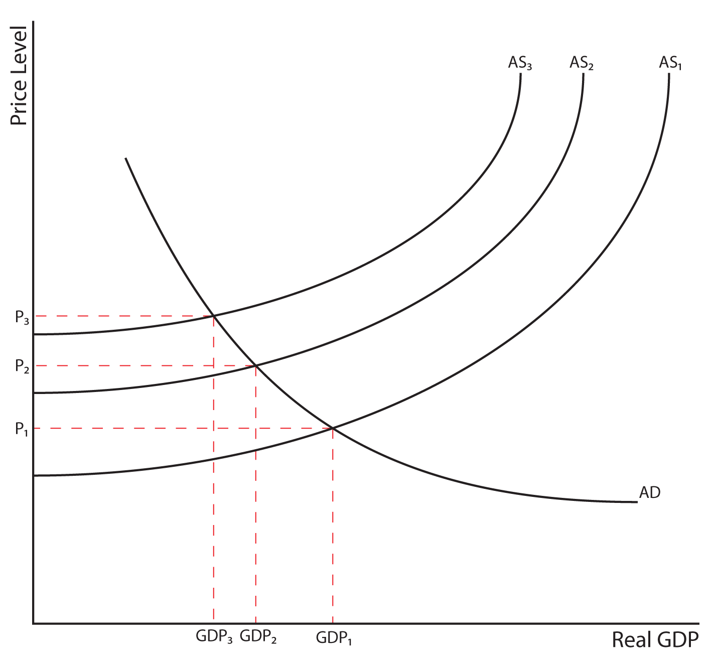
A decrease in AS will increase the Price Level and decrease Real Output. An increase in AS will reduce the Price Level and increase Real Output. The inflation that is associated with a decrease in the AS is called Cost-Push Inflation. During the 1970s, a variety of factors shifted the AS curve to the left. The high inflation that was combined with a stagnant economy (low levels of output and high unemployment) gave rise to the term Stagflation.

When Ronald Reagan was elected President in 1980, the inflation rate was 13.5% and the unemployment rate was 7.5%. Reagan employed supply side policies that were designed to shift the AS curve to the right and reduce both inflation and unemployment simultaneously. Only by supply side policies can you decrease both inflation and unemployment at the same time. By the time that Reagan left office eight years later, the inflation rate in the economy was 4.1% and the unemployment rate of 5.3%.

Section 08: The Recessionary and Inflationary Gaps Revisited

When the AD curve intersects the AS curve in the Keynesian Range or in the Intermediate Range such that output is below Qf, there exists what is called a recessionary gap. The gap represents the amount of government spending that would be necessary to shift the AD to the right enough to bring output to Qf. In the Keynesian Model, the magnitude of the shift in AD will depend on the size of the multiplier. For example, if the multiplier is 2.5, a 40 million dollar increase in government spending would shift the AD curve to the right by 100 million dollars. So if the AD needs to be shifted to the right by 100 million dollars to get to Qf and the multiplier is 2.5, there is a 40 million dollar recessionary gap. Conversely, if the AD needs to be shifted to the left to get to Qf, there is an inflationary gap and the same multiplier principles would apply.

The changes in government spending that would close an inflationary or recessionary gap are applications of fiscal policy, which is the topic of our next lesson.