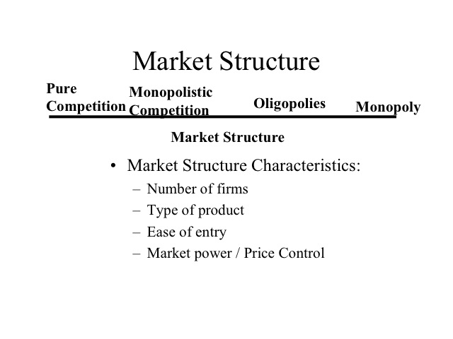
Market Structure Characteristics
Think of the different products or services that are purchased. If you asked someone what brand of cars or shoes they purchase, it is likely that they could tell you the brand name. But if you asked them what brand of flour, milk, or eggs they purchase, the answer might be, I don’t know, I just buy whatever is cheapest. How consumers view a particular product or service influences the market power and behavior of a business or producer.
In the next few sections we will discuss four different market structures and their behavior. You can think of businesses being on a continuum with one extreme being perfect competition to the other extreme being monopolies. While few businesses are actually at either extreme, it is useful to look at the two extremes for comparison purposes. In between the two extremes are most businesses, which fall into the categories of monopolist competition and oligopolies. When examining the structure of a market, we focus on the differentiating characteristics: number of firms, type of product, ease of entry, and market power or price control.
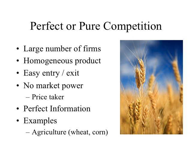
In the perfect or pure competition market, there are a large number of firms each producing the same product (as called a standardized or homogeneous product). Since the number of firms is very large, no one firm can influence the market price, thus each firm has no market power and each is a price taker. We also assume that there is perfect information, meaning everyone knows what price is being charged in all markets. The barriers to entry are low, so it is easy for other firms to get into or out of the market.
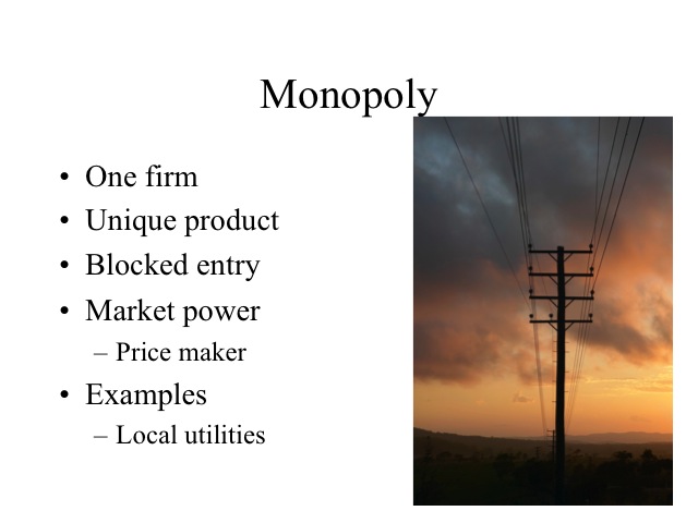
On the other end, a monopoly has only one firm and produces a unique product that has no close substitutes. Entry into the industry is blocked which allows the firm significant price control and market power.
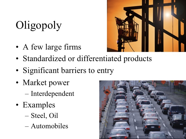
Oligopolies have a few large firms and may produce either a standardized product, such as steel, or a differentiated product, such as automobiles. There are significant barriers to entry which limit the number of firms that can enter the market often due to the cost structure of the industry. Since there are only a few firms, the market power of a firm depends on the actions of the other firms in the industry.
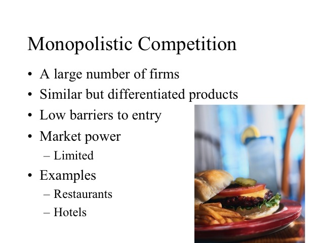
There are a large number of firms with lower barriers to entry in monopolistic competition. The products they produce are unique to the firm but very similar to those produced by other firms. For example, only one firm produces the Big Mac or the Whopper but there are many products similar to each. Since the barriers to entry are low and the products each firm produces are similar, firms have a limited degree of market power.
Although each firm does not ideally fit in one of the four market structures, all firms can be placed along this continuum based on their characteristics. Given the characteristics of the industry, we will study how firms in that industry behave.
Section 02: Pure Competition in the Short Run
Pure Competition
How do firms in pure competition behave in the short run when at least one of their inputs is fixed? Agriculture commodities are our closest example to a purely competitive market. Commodities such as wheat, corn, milk, and eggs from one farm are viewed by consumers to be same as those same commodities from other farms. If the grade A large eggs from company X tastes just like the grade A large eggs from company Y then the consumer will purchase whichever one is cheapest.
In pure competition there are a large number of firms such that no one firm can influence the price. To help put this in perspective, let’s look at wheat farming. According to the 2007 Census of Agriculture, nationally the average farm size of all types of farms is 418 acres. So a farm that had several thousand acres of wheat would be considered a large farm. However, given that there is approximately 60 million wheat acres planted domestically each year, even a farm of 10,000 acres would only represent .016 percent of the total, which would not be enough to influence the market price.
References:
http://www.ers.usda.gov/StateFacts/US.htm
http://www.ers.usda.gov/briefing/Wheat/2005baseline.htm
http://www.msu.edu/user/hilker/outlook.htm#wheat
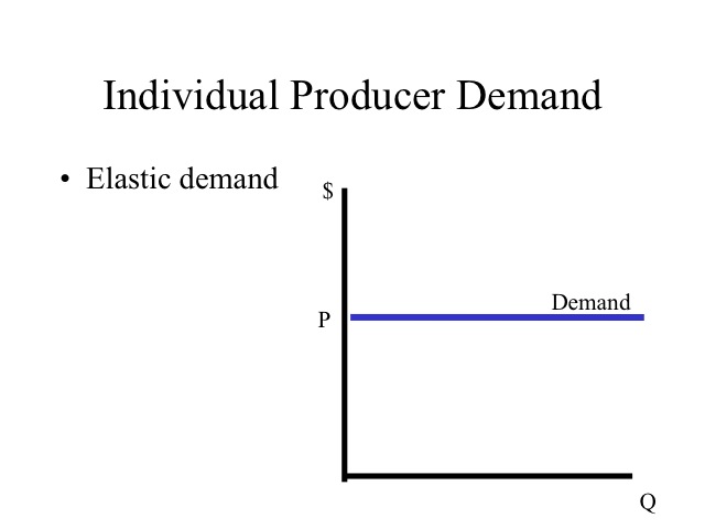
Since each producer makes up a very small portion of the total market, no one producer can influence the price. The demand curve faced by each producer is completely elastic (horizontal). Producers are said to be price takers. An individual producer can sell as much as he has the ability to produce at the going market price, but if he tries to raise his price, even slightly, demand goes to zero. Consumers view each bushel of wheat as being the same as the next, so their only concern is the price.
In an efficient market where all goods are identical, the law of one price would indicate there should be one price for the commodity if transaction costs were zero. In other words, if a commodity such as wheat could be moved for no cost from one place to another, we would expect there to be one overall price emerge. Since transactions costs are positive, the difference that we would expect to see in the price of commodity would be based on the supply and demand of the commodity in each area and the cost of shipping the commodity. In perfect competition, we assume there is perfect information, in other words, we know exactly what price wheat is being sold for everywhere. If wheat is selling for a higher price in a neighboring town such that a farmer could increase his profits by taking his wheat there, the supply of wheat in that town would increase lowering the price and the price of wheat in the farmer’s town would decrease driving the price to be same in the two towns except for the transaction costs.
Why do we see industries that produce a commodity advertise but we typically don’t see individual firms advertise?
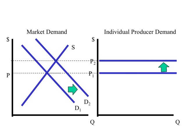
Producers are able to sell all the product they can produce at the going market price and have no ability to raise price through advertising, thus they have no incentive to incur the cost of advertising. However, the price that the individual producer receives is based on the equilibrium market price which does have a downward sloping demand curve. Successful advertising as an industry shifts the market demand curve to the right, leading to a higher price for each individual producer. Thus there is a benefit from advertising collectively but not individually. There is an incentive for individual producers to be free riders, allowing others to pay for the cost of advertising while all reap the benefits. To avoid this problem, most marketing takes place through associations or marketing boards that force all producers to contribute to the marketing fund. For example, a certain amount is charged for every hundred pounds of milk sold to pay for advertising milk. Other examples of industry advertising include the beef, pork and egg industries.
Since producers have no control over the price of the good, their only decisions are to determine if they should produce and if so, how much. With the goal of maximizing profits, firms in pure competition must evaluate both the price they can sell the good for and the respective costs of producing the goods.
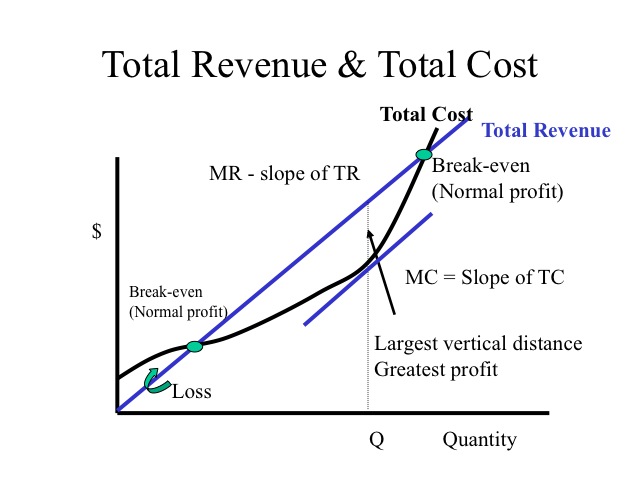
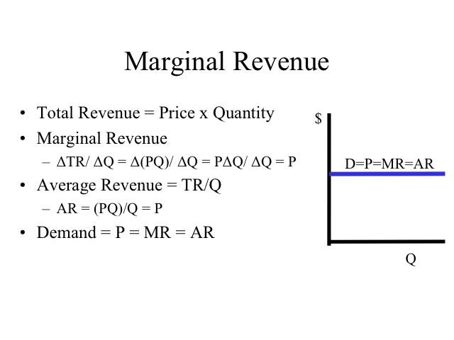
Profit is equal to total revenue minus total cost, so the profit maximizing output level is where there is the greatest vertical distance between total revenue and total cost. At that point, the slope of the total revenue line is the same as the slope of the total cost curve. Note that since the price remains constant at each quantity, the total revenue line is a straight line with a slope that is equal to the price of the good. The slope of the total revenue is the marginal revenue and the slope of the total cost curve is the marginal cost. Since at the profit maximizing quantity the slopes of both curves will be the same, profits are maximized where marginal revenue equals marginal cost.
Marginal revenue is the additional revenue generated from selling one more unit of output. The formula is the change in total revenue divided by the change in quantity or output. Total revenue is the price times quantity and since the price is constant for each good sold, the marginal revenue in a purely competitive market is simply the price of the good. Thus in pure competition, the demand is equal to the marginal revenue which is also equal to the average revenue.
A firm will always maximize profits or minimize losses, if it produces where the marginal revenue equals the marginal cost. A firm evaluates if incurring the additional cost is offset by the additional revenue generated. For example, at 30 units of output is it worth 20 cents more to get 65 cents? Certainly. The firm will continue to increase output up to the point where the marginal cost is equal to the marginal revenue, which in our example occurs at 70 units of output. If we produced 80 units, the marginal cost of 70 cents would be greater than the marginal revenue of 65 cents and profits would decline.
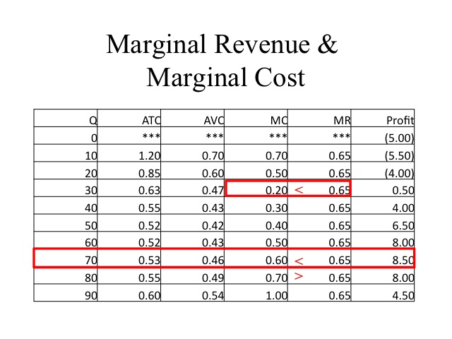
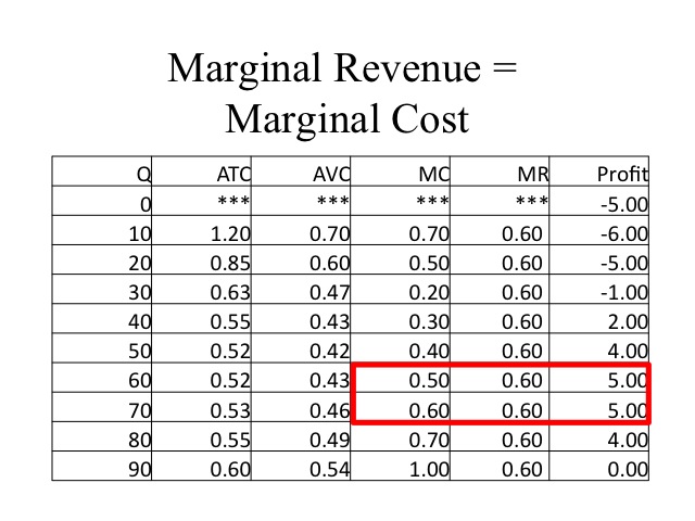
If we go to the exact quantity where marginal revenue equals marginal cost, then for the last unit produced there was no increase in the profits. For example, at 70 units the marginal revenue and marginal cost are 60 cents and the profits of 5 dollars is the same as the profits at 60 units. However, by following the rule of going to the point where marginal revenue equals marginal cost, there will not be another quantity that will yield greater profits.
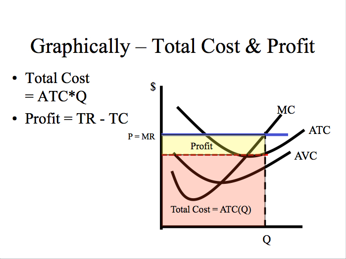
For pure competition, to solve graphically, we combine our costs curves with the demand curve, which is also our marginal revenue curve and find the quantity where marginal revenue equals the marginal cost. The area representing total revenue, which is price times quantity, is shown in the shaded box.
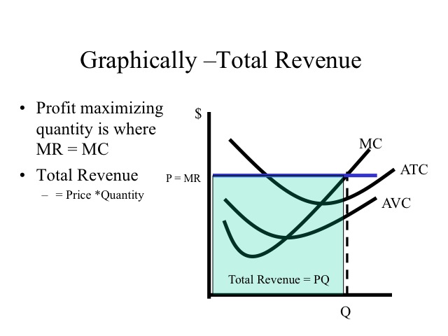
The total cost can be computed by taking the average total cost at the profit maximizing quantity times the quantity. Profit is total revenue minus total cost and is represented by the upper shaded box.
Why do some businesses open at 9 am and close at 5 pm while others stay open till 11 pm, or are open all night? Would it ever be a wise decision for a business to continue to stay open, in the short run, if it is losing money? The answer depends on the firm’s fixed costs, the additional revenue it generates by being another hour, and the additional costs (variable costs) it incurs by being open another hour.
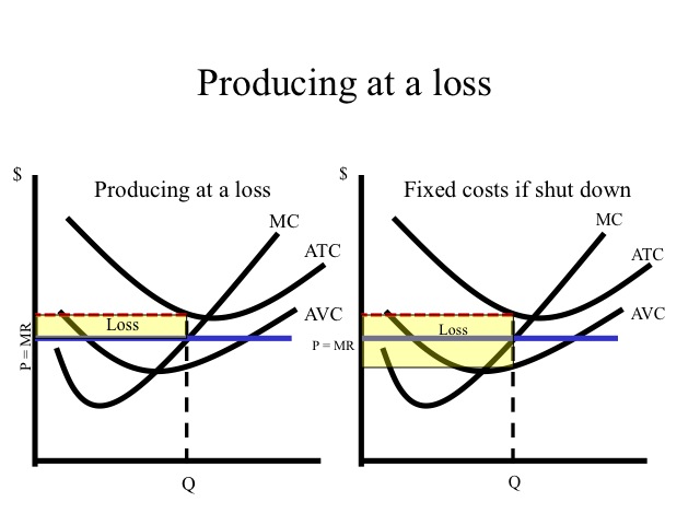
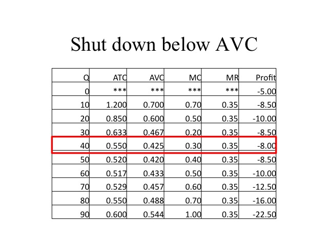
Recall that in the short run, firms have fixed costs that must be paid regardless. Thus if a firm can cover its variable costs and still have revenue to contribute to its fixed costs, it loses less money by producing than by shutting down. Our rule of producing where marginal revenue equals marginal cost still applies, but since price is below ATC the firm’s loss is represented by the area below ATC and above the demand curve. Even though the firm continues to produce, the amount of production is less than when the price was higher.
The average fixed cost is the vertical distance between average total cost and average variable cost, thus if the firm decided to shut down the firm would still have to pay the total fixed costs, which is represented by the shaded area in the graph on the right.
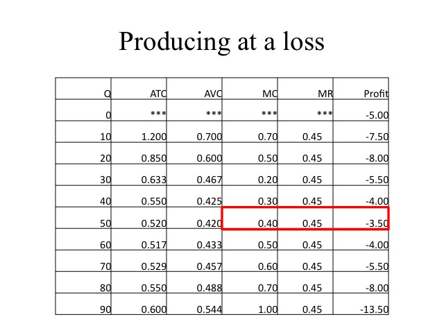
As demonstrated in the table, if the price is below average total cost but above average variable cost, losses are minimized by producing 50 units and incurring a loss of $3.50. If the firm shut down, it would still have to pay fixed cost of five. Since average variable costs at 50 units is 42 cents and the price is 45 cents, it covers the variable costs and contributes three cents on each unit toward the paying the fixed costs. Three cents times 50 units is $1.50 which is the amount the firm has reduced their loss by producing instead of shutting down.
If the price drops below the average variable cost, the firm is unable to cover even the variable cost and can reduce the loss by shutting down and paying only the fixed costs.
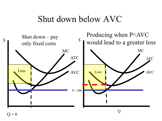
The firm losses less money by shutting down and only incurring the fixed costs of five dollars than by producing and losing even more.
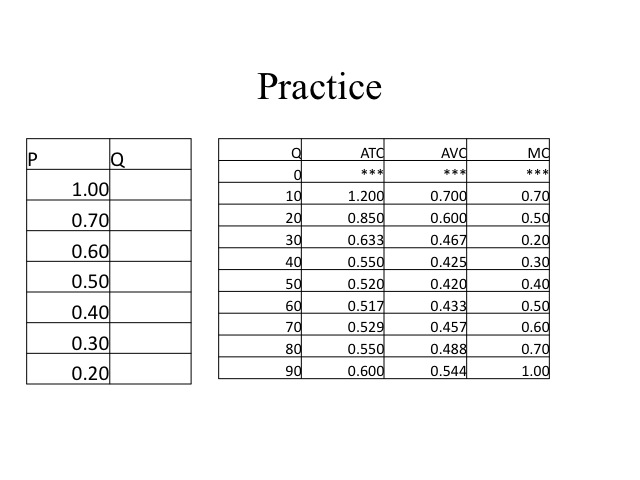
Practice
Determine the profit maximizing output level for the firm at each of the respective prices and calculate profit.
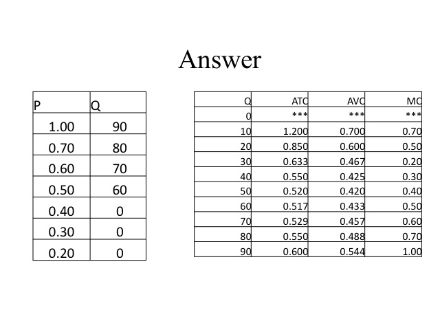
Answer
Determine the profit maximizing output level for the firm at each of the respective prices and calculate profit. At 40 cents and below, the average variable cost is greater than the price so the firm is better off to shut down and only pay the fixed costs.
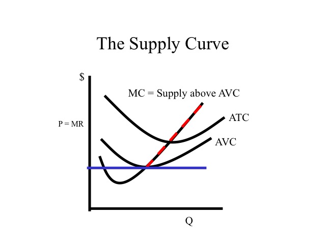
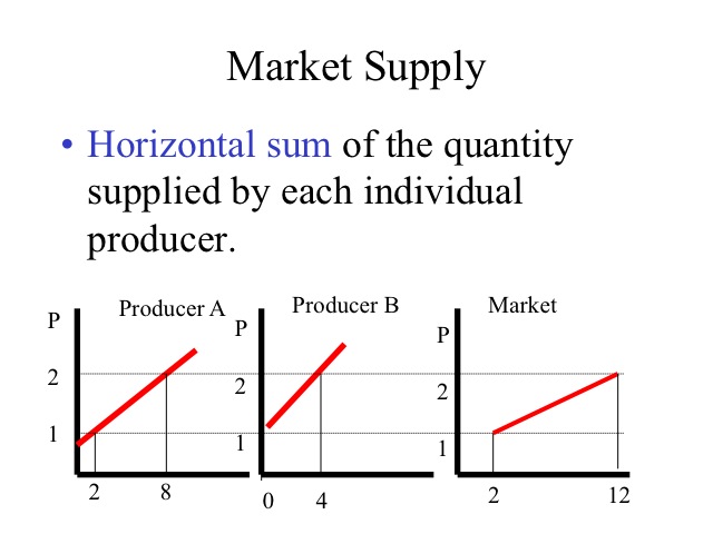
Since profit maximization takes place where marginal revenue is equal to marginal cost, in pure competition the firm’s supply curve will be it’s marginal cost curve above the average variable cost.
The horizontal summation of the individual firm’s supply curves yields the market supply. For example, if we only had two firms in the market and at one dollar, Producer A would supply 2 units and B would supply zero, then the market supply at one dollar would be two. At two dollars, A provides 8 units and B provides 4 making the market supply 12.
Practice
A farmer just before harvest suffers a damaging hail storm which cuts his expected wheat yield to only 20 bushels per acre which he can sell for 4 dollar per bushel. The farmer has already invested 300 dollar per acre in seed, fertilizer, and other expenses. To have someone custom harvest the crop will cost him an additional 60 dollars per acre. The alternative is to not harvest and plow the crop under. Assume the plowing costs are the same, regardless if he harvests or not and that there is no crop insurance. Should the farmer harvest or just plow the crop under? Explain why?
Answer
The $300 per acre the farmer has already spent is a sunk cost. Fixed costs are sunk and should not be considered in our decision in the short run. So the question is to determine if the additional revenue generated from harvesting will cover the additional expense. By harvesting, he will make 20 per acre, and although he is still going to lose money, he will only lose 280 per acre as opposed to the 300 per acre if he doesn’t harvest.
Key Points for Pure Competition in the Short Run
Here are a few key points to remember for pure competition in the short run.
1. Demand is completely elastic for an individual firm but not for the industry.
2. For the individual firm, price equals marginal revenue.
3. Profits are maximized or losses minimized by producing where MR = MC, above AVC.
4. If price is below AVC, the firm should shut down and pay only the fixed costs.
5. The supply curve of an individual producer is the marginal cost curve above AVC.
Section 03: Pure Competition in the Long Run
How Firms in Pure Competition Behave
How do firms in pure competition behave in the long run?
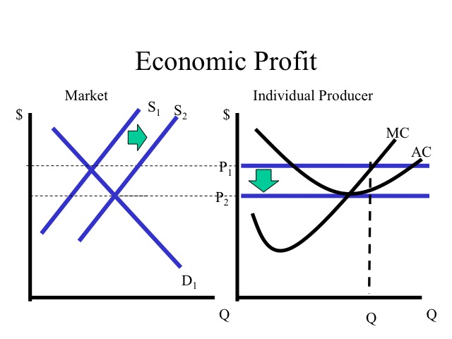
With low barriers to entry, if the industry is making an economic profit there is an incentive for other firms to enter the business. As more firms enter, the supply of the product increases, driving down the price and reducing the profits. This will continue until the firm’s economic profit is reduced to zero. At an economic profit of zero, firms are still earning a normal profit, which is a return sufficient to maintain the resources in their current use. Recall that in the long run, all inputs are variable. It is for this reason that we don’t have fixed costs and that we make no distinction between variable costs and total costs.
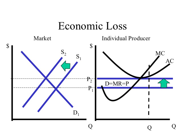
If firms are sustaining economic losses, they will eventually exit the industry due to the high opportunity costs. As firms leave, the market supply shifts to the left and the price rises reducing the losses.
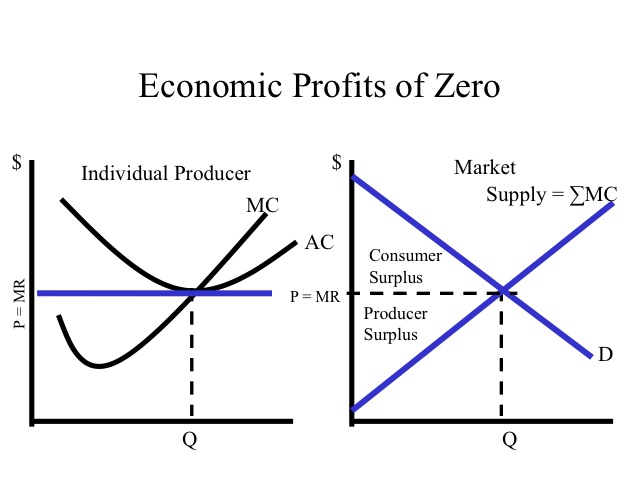
In the short run firms may earn economic profits or losses, but in the long run economic profits can be expected to be zero and firms will earn only normal profits. In the long run, firms are both productively and allocatively efficient. Since the marginal cost curve intersects the average cost curve at the minimum, and firms produce where marginal revenue is equal to marginal costs, firms will be productively efficient (recall productive efficiency means “least cost” since we are at the minimum ATC, we must be at least cost). Moreover, in this market there is a strong incentive to adopt new technologies which reduce costs. Since there is easy entry into the market, if a firm fails to adopt the new technologies that reduce costs, it will eventually be forced out of the market since it is not producing at the lowest average cost.
Firms are also allocatively efficient and produce where the price is equal to the marginal cost. In the market graph on the right, demand reflects the willingness to pay by consumers and the supply curve reflects the marginal cost. At the quantity produced, economic surplus which is the area of consumer and producer surplus is maximized. The purely competitive market is a useful benchmark when examining other market structures, because it is both productively and allocatively efficient.
Practice
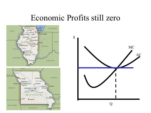
The state of Illinois is known for having some of most fertile soils in the nation, while parts of Missouri have marginal (low productivity) soils. If the yield per acre is greater in Illinois and the price of the output (corn, wheat, soybeans) is the same for both states, will Illinois farmers make greater profits than Missouri farmers in the long run? Explain why or why not?
Although Illinois farms would be expected to have higher yields, we would expect the economic profits in both states to be zero in the long run. The price will be the same for all farms, but we would anticipate that land in Missouri would sell or rent for less than land in Illinois since it is more productive.
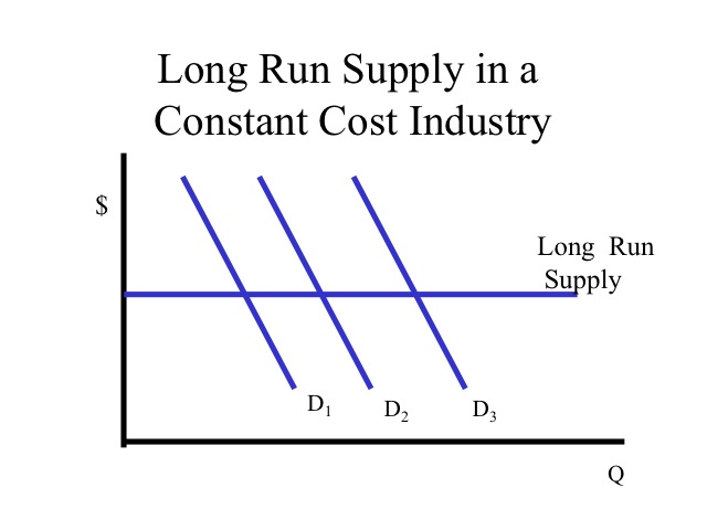
If the prices of the resources do not change as their demand changes, then the long run average cost curve for individual firms remains the same as market production increases and decreases. This would likely be the case, if an industry makes up a relatively small portion of the overall demand for the inputs. If this were the case, the long run supply curve would be horizontal and the price of the good would remain constant as output expands or contracts.
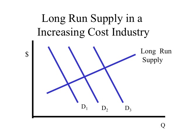
Most industries have increasing costs such that as the quantity of the output increases, production costs also increase. Likewise if output falls, the price of the inputs will also decrease due to the decreased demand. In our wheat example as output increases, production costs such as the price of farmland increases shifting the average cost curve upwards. This would result in an upward-sloping long-run supply curve.
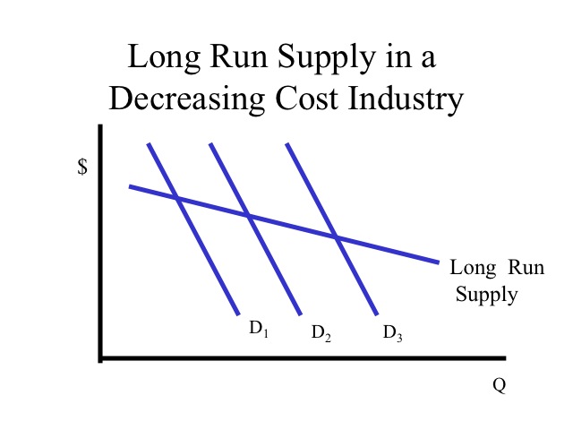
In a decreasing cost industry, the long run supply curve is downward sloping since as output increases and new firms enter, production costs decline. The computer industry is an example of a downward sloping supply curve, since as the number of computers produced increased, the price of inputs, such as chips, decline.
Key Points for Pure Competition in the Long Run
1. Short run economic profits (losses) leads to firms entering (exit) the industry.
2. Ease of entry will cause long run economic profits to be zero.
3. In the long run, purely competitive firms will be both productive and allocatively efficient.
4. Economic surplus is maximized in pure competition.