Section 01: Consumer Behavior
In this section, we are going to take a closer look at what is behind the demand curve and the behavior of consumers. How does a consumer decide to spend his/her income on the many different things that he/she wants, i.e., food, clothing, housing, entertainment? We assume that the goal of the consumer is to maximize his/her level of satisfaction or joy, constrained by his/her income.
Economists use the term utility as a measure of satisfaction, joy, or happiness. How much satisfaction does a person gain from eating a pizza or watching a movie? Measuring utility is based solely on the preferences of the individual and has nothing to do with the price of the good. Let’s do an experiment in utility.
Step 01: Get some of your favorite candy, pastries, or cookies.
Step 02: Take a bite and evaluate, on a scale from 0 to 100 (with 100 being the greatest utility), the level of utility from that bite. Record the marginal utility of that bite (i.e., how much you get from that one additional bite).
Step 03: Repeat step 02. It is important to be consistent with each unit consumed, i.e., the same size and no drinking milk or water part way though. When you run out of candy or your marginal utility goes to zero you can stop.
Law of Diminishing Marginal Utility
The law of diminishing marginal utility states that as more of the good is consumed, the additional satisfaction from another bite will eventually decline. The marginal utility is the satisfaction gained from each additional bite. As more of the good is consumed, we gain less additional satisfaction from consuming another unit. Thus even if a good were free and you could consume as much as you wanted, there would be a limit to the amount you would consume due to the law of diminishing marginal utility.
Summing the marginal utilities gives us the total utility. For example, let’s say the first chocolate was an 85 and the second chocolate had a marginal utility of 79, then the total utility from consuming two chocolates is 164. The total utility from consuming three chocolates is 85+79+73 = 237. As long as our marginal utility is positive our total utility increases although with diminishing marginal utility it increases at a decreasing rate.
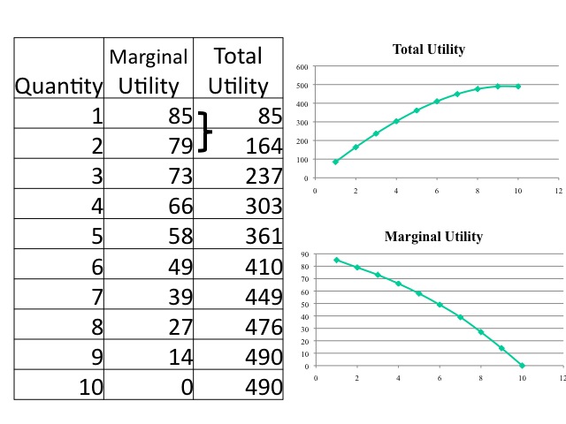
Can marginal utility be negative? Yes. At a holiday dinner, you may overeat and suffer from indigestion afterwards to a point where you regret having eaten too much, but at the time of the dinner, you expected greater utility from eating the last of the meal. We would not willingly consume an item that gave us negative marginal utility. Then why would an individual stuff themselves during a hot dog eating contest where clearly the last hot dogs consumed are making them worse off? Although the marginal utility from the last hot dog itself makes the person worse off, the utility from winning the contest is greater making the marginal utility positive.
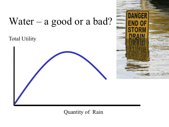
The marginal utility of an item can change. For example, during a drought water provides a high positive marginal utility, and with more rain the marginal utility declines. At some point, there is too much rain, it turns from being a good utility to a bad one and the marginal utility of more rain, when it is already flooding, is negative.
Utility values can be determined by an individual ranking his/her preferences from least preferred to most preferred. The resulting ranking or utility values are subjective or individual. They are also ordinal rather than cardinal. Ordinal means that the utility values simply define a ranking of preferences rather than an actual cardinal measurement.
Imagine a class has 10 students in the class and the teacher lined the students up according to height. He then numbered them off according to height, assigning the shortest student a 1 and the tallest student a 10. Is it true that student number 4 is twice tall as student number 2? Of course not. All we know from the ranking is that student number 4 is taller than student number 2. Now, imagine that in another class another teacher has also ranked 10 students according to height. Is it true that student number 10 from the second classroom is taller than student 1 from the first classroom? We cannot say since the ranking is only valid within a particular course. In order to say a student is twice as tall as another student or to be able to compare students between classes, we would need a cardinal measure of height like inches or centimeters.
Since utility is ordinal and not cardinal we cannot make interpersonal comparisons of utility. Does a rich person value a dollar more or less than a poor person? While some would say that a poor person likely has more unmet needs and thus he would value the dollar more. The answer is that it all depends on the preferences of the individuals. A poor person may prefer to live a more simplistic life and place a lower value on having an extra dollar than a rich person who has a “love of money” (1 Timothy 6:10). We simply cannot make such an interpersonal comparison of utility.
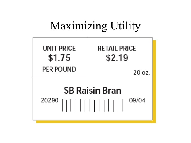
So how does the consumer decide what to purchase? Unfortunately everything has a price and consumers only have so much money to spend. Consequently consumers try to spend the limited money they have on what will give them the greatest amount of satisfaction. The decision rule for utility maximization is to purchase those items that give the greatest marginal utility per dollar and are affordable or within the budget. Many grocery stores provide a tag that indicates the price per pound for the good. This allows consumers to compare the cost per pound for different brands or different sizes. The same concept is used for maximizing utility but we divide the marginal utility by the price to get the marginal utility per dollar.
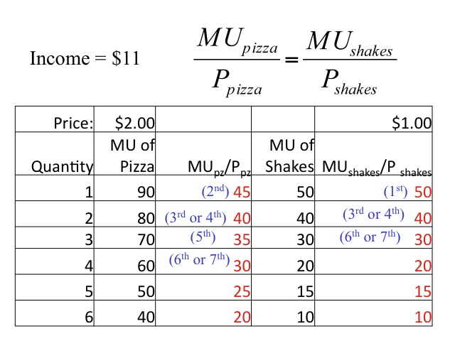
Let’s say that we eat only two goods: milk shakes and pizza where the price of each slice of pizza is $2 and the price of each shake is $1 and we only have $11 to spend. Since the price of each good is different we need to divide the marginal utility by the price to allow for a common comparison. We then compare the marginal utility per dollar for pizzas verses shakes. For the first unit the marginal utility per dollar of a shake is 50 compared to only 45 for the pizza, so we would purchase the first shake. We then compare the marginal utility per dollar of the first pizza (45) to the marginal utility per dollar of the second shake (40) and purchase the first slice of pizza. If the marginal utility per dollar is the same for the two goods and we have income to purchase both then we would do so, as seen in the second slice of pizza and the second shake.
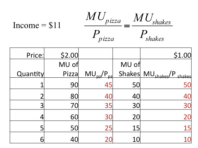
We continue to allocate on budget on those goods that yield the highest marginal utility per dollar. In this example, we would purchase four slices or pizza and three milkshakes and spend our entire budget of $11. The total utility from this purchase would be the sum of the marginal utilities: 50 + 90 + 80 + 40 + 70 + 60 + 30 = 420. At the last items purchased the marginal utility per dollar spent on the two goods is the same, no other combination of pizzas and milk shakes will give us greater utility given our budget.
Practice
Here is your chance to practice. Holly has $20 to spend on either movies or bowling and wants to maximize her utility. Complete the table and determine how many movies and rounds of bowling will maximize her utility.
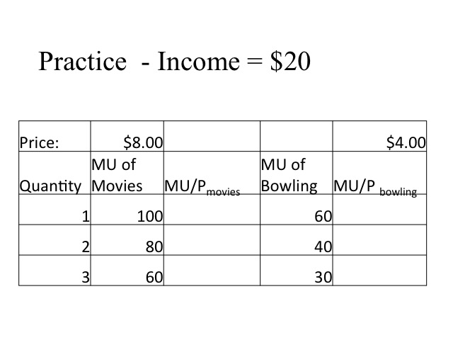
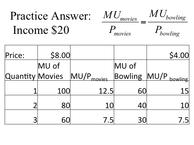
Our first step is to divide the marginal utility of each item by the price. With an income of $20 she is limited in what she can purchase. Since the marginal utility per dollar for bowling (15) is greater than the marginal utility of the first movie (12.5) she would initially go bowling, spending $4. Comparing the first movie (12.5) to the second round of bowling (10) she would go to the movie spending an additional $8 and a total of $12. The decision is a little harder. Holly has eight dollars still to spend and the marginal utility per dollar is the same for each good. If she chooses the movie she will spend all eight dollars, but if she goes bowling she will spend four dollars and still have four to spend. We have assumed that she wants to spend all her money and gains no utility from holding the cash. Since she can’t afford to buy another movie but would instead by a third round of bowling, which only has a marginal utility per dollar of 7.5. Thus we see that to maximize her utility, she would purchase one round of bowling and two movies giving her a total utility of (60 + 100 + 80) = 240. Recall our decision rule is to have the marginal utility per dollar spent on the last items be the same for all goods. In this case, we are unable to have that exactly but we try to get as close as possible. There is no other combination that would give us greater utility given our income.
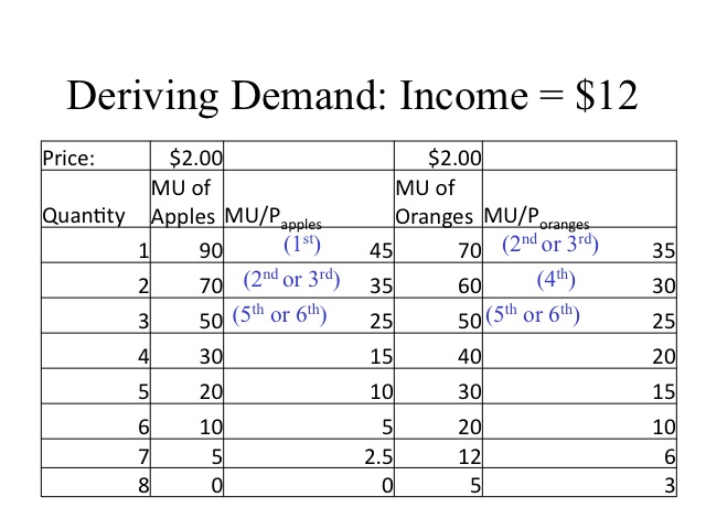
Knowing how the consumer behaves allows us to derive a demand curve. Let’s say that Suzette eats either an apple or an orange as a snack. She has $12 to spend. Given that each fruit costs two dollars, she will maximize her utility by purchasing 3 apples and 3 oranges. If we are looking at the demand for oranges, this will give us one point on the demand curve. At a price of $2.00, the quantity demanded of oranges is 3.
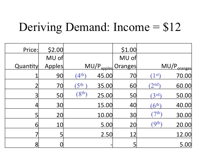
Recall that as we move along the demand curve, the only thing that changes is the price of the good (ceteris paribus or holding all else constant). If the price of oranges decreases to $1, the quantity of oranges demanded increases to 6.
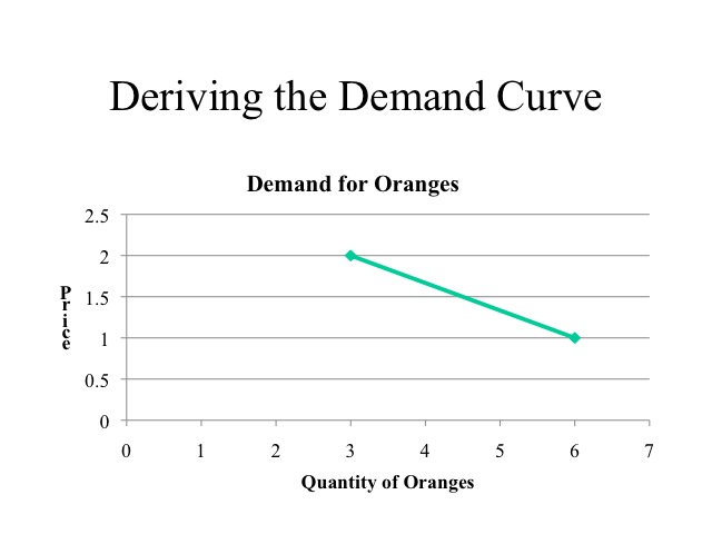
We can plot the two points and create a demand curve for oranges. At a price of $2 the quantity demanded is 3 and at a price of $1 the quantity demanded is 6. Recall that the demand curve reflects the marginal benefit or the willingness to pay of the consumer.
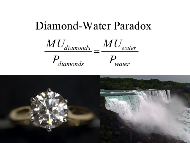
The demand curve can be seen in the diamond-water paradox. Why does water that is essential to sustain life cost so much less than diamonds that are atheistically pleasing, but are relatively unnecessary? Recall that price reflects the scarcity of a good. Overall, the supply of water is relatively abundant while the supply of diamonds is relatively limited. Thus the price we pay for water is low compared to the price of diamonds.
Is it logical for someone who is maximizing his utility to purchase both water and diamonds? When deciding what to purchase we compare the marginal utility divided by the price. With lots of water consumption, the total utility of water is very large but the marginal utility of the last gallon consumed is relatively low. Few diamonds are purchased so while the marginal utility is very large, say the diamond ring you just purchased for your future spouse, the total utility is low since few diamonds are purchased.
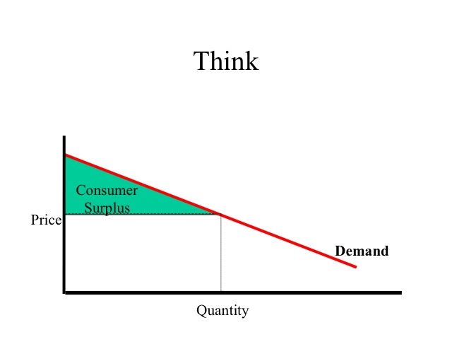
Knowing that individuals experience diminishing marginal utility, how do businesses react? Recall that consumer surplus is the area below the demand curve but above the price. Think of some examples of how businesses react given the law of diminishing marginal utility.
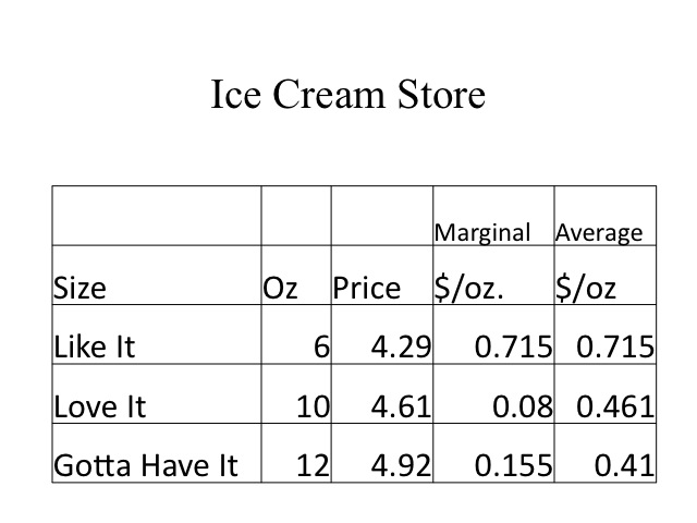
One example is the price per unit based on package size. An ice cream store has three different serving sizes - a 6, 10, and 12 ounce cup. The price of the smallest size, "Like It," is $4.29 or 71.5 cents per ounce. For just 32 cents more, one can have four more ounces, "Love It," making the marginal cost per ounce 8 cents and the average cost per ounce 46 cents. Upgrading to the "Gotta Have It" size adds an additional two ounces with only 15.5 cents per ounce more and an average cost per ounce of only 41 cents. Certainly the large size is cheaper per ounce, but not everyone wants to eat that large of a serving. For those only wanting a small serving, the store takes advantage of their greater willingness to pay for that portion size. Whether its ice cream, eggs, milk, popcorn, or cereal, it is common practice to charge a higher price per unit for a smaller package size. However it pays for consumers to do the math since businesses will at times charge a higher price on the larger packages size. If customers believe that bigger is always cheaper and fail to do the math, they may get caught paying a higher price per unit.
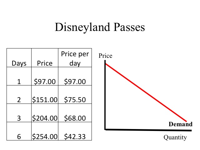
Services often follow a similar pricing scheme with lower average prices for more frequent attendance. For example, below are the prices for the “hopper pass” at Disneyland. Tickets to sporting events follow a similar pricing approach with the per game price being lower if multiple games are purchased, such as the season pass.
Regular prices as of 1/18/10
http://disneyland.disney.go.com/disneyland/en_US/reserve/ticketListing?name=TicketListingPage
Consider this example. You are on a long airplane ride, seated next to an eccentric looking woman and a businessman. Halfway into the flight, the woman says to you and the businessman, that she is very rich and bored of flying. To break up the monotony, she offers you and the businessman a chance to split $5,000. The rules are as follows: the businessman makes an offer of how to split the money and you either accept or reject. If you accept, you get the agreed upon split. If you don’t, you both get nothing. This is a one time offer. The businessman thinks and offers the following split $4,995 for him and $5 for you. Do you accept or reject the offer? Why?
The answer to these questions will vary among individuals. Some will accept stating they have five dollars more than they did before. Others will reject the offer, saying that it is worth at least five dollars to them to deny they businessman the $4,995. Remember that when we talk about utility, it includes not only monetary items but also the nonmonetary.
In The Theory of Moral Sentiments, Adam Smith wrote: "How selfish soever man may be supposed, there are evidently some principles in his nature which interest him in the fortune of others and render their happiness necessary to him though he derives nothing from it except the pleasure of seeing it.” Remember that utility is derived from many different areas including service and philanthropic acts.
Reference: http://www.econlib.org/Library/Enc/bios/Smith.html
Section 02: Indifference Curves and Budget Constraints
Indifference Curves
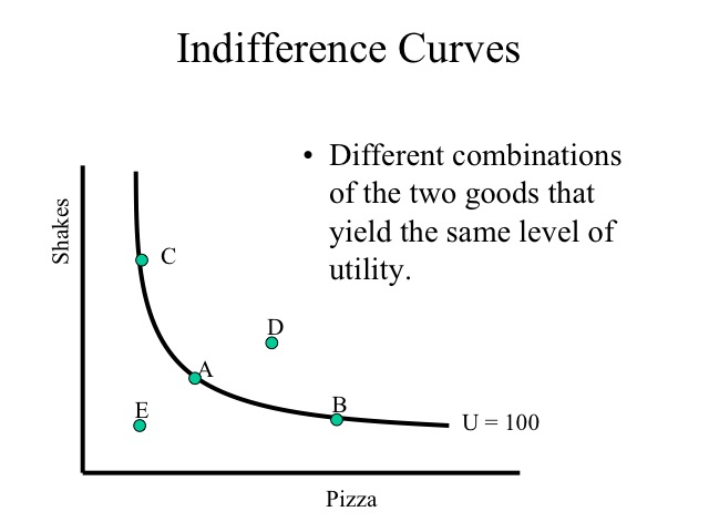
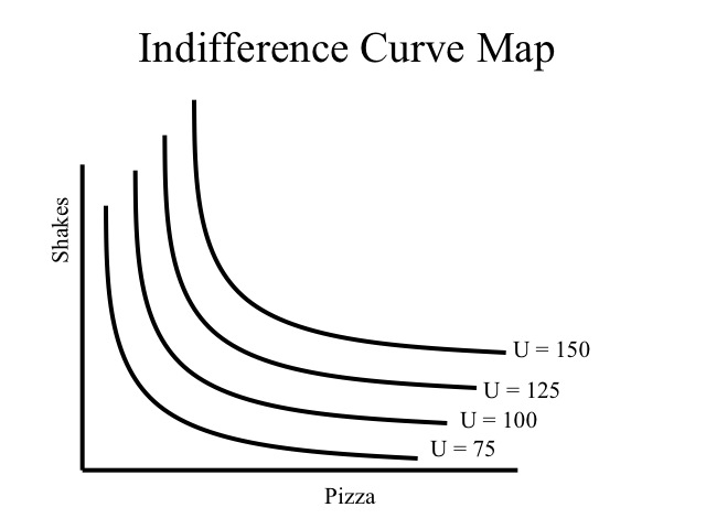
Indifference curves and budget constraints allow for a more in-depth analysis of demand. For modeling purposes we will look at the two goods. An indifference curve shows the different combinations of the two goods that yield the same level of utility, independent of the price of the goods. Due to the law of diminishing marginal utility, the indifference curve between the two goods is convex to the origin. All combinations of the two goods (pizza and shakes) that are on the indifference curve (A, B, and C) yield the same level of utility, say Utility = 100. Having more of good, yields a higher level of utility (combination D) and having less of the goods yields a lower level of utility (combination E).
An indifference curve map shows the family of indifference curves. There could be an infinite number of indifference curves that would reflect the level of utility at different combinations of the two goods. Just as a line on a topographical map indicates the different points that are at the same elevation, the different points along an indifference curve, indicate that same level of utility.

Source: U.S. Geological Survey
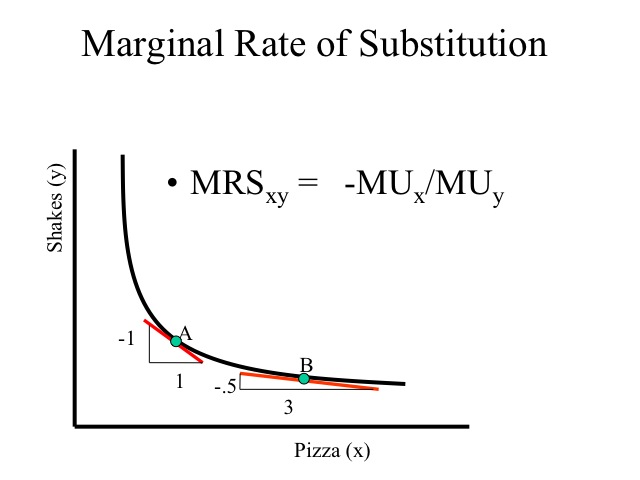
The marginal rate of substitution is the slope of the curve and measures the rate at which the consumer would be willing to give up one good for the other while maintaining the same level of utility. Thus the marginal rate of substitution reflects the ratio of marginal utilities between the two goods.
For example, at point A, the consumer would be willing to trade one shake for one additional slice of pizza. At point B, the consumer already has a lot of pizza but few shakes so the marginal utility from an additional pizza is relatively lower and the marginal utility from the shake he would have to give up would be relatively large, thus to maintain the same level of utility he would have to gain 3 pizzas to willingly give up one half a shake.
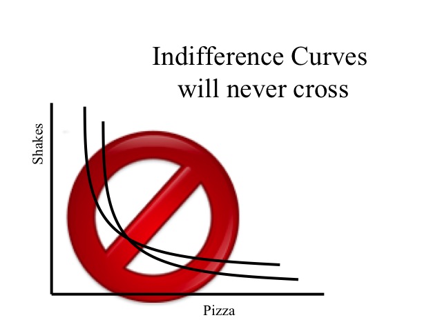
Since any combination of the two goods will only yield one level of utility at a particular point in time, indifference curves will never cross each other.
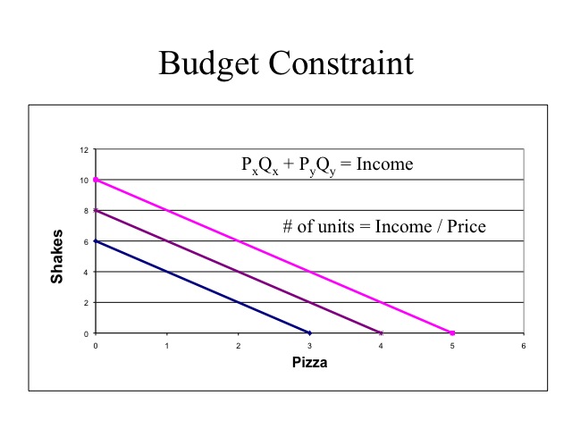
The budget constraint indicates the combinations of the two goods that can be purchased given the consumer’s income and prices of the two goods. The intercept points of the budget constraint are computing by dividing the income by the price of the good. For example, if the consumer had $8 to spend and the price of pizza was $2 and shakes were $1, then the consumer could buy four pizzas ($8/$2) or eight shakes ($8/$1). Any combination of the two goods that are on or beneath the budget constraint are affordable, while those to the outside (farther from the origin) are unaffordable.
A greater income will cause a parallel shift rightward of the budget constraint while a decrease in income will cause a parallel shift leftward.
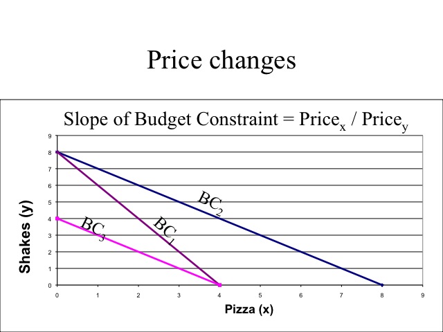
Changing the prices of the goods changes the slope of the budget constraint. If the consumer’s income is $8 and the price of pizza is $2 and the price of shakes is $1, then the budget constraint would be BC1. If the price of pizza drops to $1, then the budget constraint would rotate out on the x-axis to BC2. Alternatively, if the price of shakes increased to two dollars then the budget constraint would become BC3.
The slope of the budget constraint is the negative ratio of the prices (-Px/Py). For example, given the price of pizza (on the x-axis) is $2 and the price of shakes (on the y-axis) is $1, then the slope of the budget constraint would be -2.
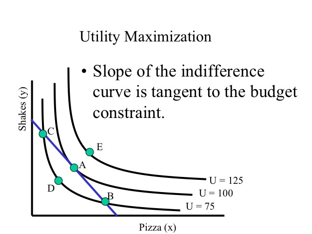
Given the goal of consumers is to maximize utility given their budget constraints, they seek that combination of goods that allows them to reach the highest indifference curve given their budget constraint. This occurs where the indifference curve is tangent to the budget constraint (combination A). Note that combinations B and C cost the same amount as A; however, A is on a higher indifference curve. Combination D yields that same utility as C and B but doesn’t use all of the income, thus the consumer can increase utility by consuming more. Combination E is preferred to combination A, but is unattainable given the budget constraint.
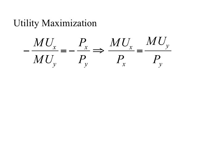
We previously mentioned that utility is maximized where the marginal utility per dollar spent is the same for each of the goods. At the point where the indifference curve is tangent to the budget constraint, the slope of the indifference curve which is the ratio of marginal utilities (-MUx/Muy) is equal to the slope of the budget constraint (- Price x / Price y). This equation can be rewritten to show that the marginal utility per dollar spent will be the same for both goods.
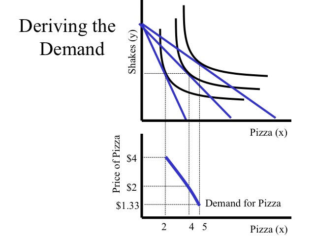
The demand curve can be derived from the indifference curves and budget constraints by changing the price of the good. For example, if the price of pizza is $4, the quantity demanded of pizza is two. If the price of pizza decreases, the budget constraint becomes flatter and the consumer can purchase more pizza, say the price of pizza drops to $2 and consumer purchases 4 units. If the price drops to $1.33, the quantity demanded increases to 5. Plotting each of the price and quantity demanded points creates the demand curve for pizza.
Income and Substitution Effects
When discussing why the demand curve is downward sloping, we outlined the substitution effect and income effect. We can observe the changes in quantity demanded along the demand curve due to the change in price; however, the indifference curves and budget constraints can help us analyze the size of the income and substitution effects.
For example, say the consumers income is $15 and the price of apples is $1 and the price of oranges is $3. At these prices the consumer purchases six apples and three oranges. When the price of oranges falls to $1, the consumer purchases eight apples and seven oranges. Thus on the demand curve for oranges, the consumer purchases three oranges when the price is three dollars and seven oranges when the price is one dollar.
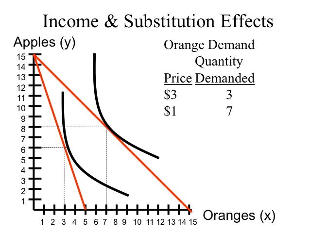
Bringing the new budget constraint back to the original indifference curve allows us to break down the income and substitution effects. Since the slope of the budget constraint reflects the ratio of prices, the substitution effect is the increase in the number of oranges that would be purchased given the new prices, while staying on the original indifference curve that is moving from point A to point B. The movement from point B to point C is the income effect, the additional consumption of oranges due to the increased purchasing power. With a decrease in the price of oranges, the relative price of apples has increased and fewer apples would be consumed due to the substitution effect; however, due to increased purchasing power, more apples are purchased as well as more oranges.
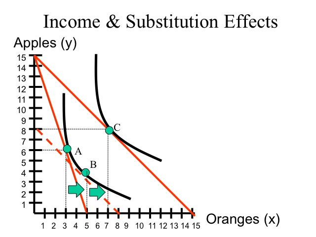
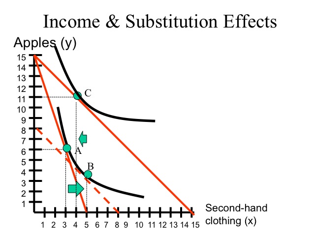
Recall from our elasticity discussion that the income elasticity for an inferior good is negative. For example, as income rises the demand for used clothing decreases. Looking at second-hand clothing on the x-axis, as the price declines the substitution will be positive (movement from point A to point B); however, the income effect (movement from B to C) will be negative.
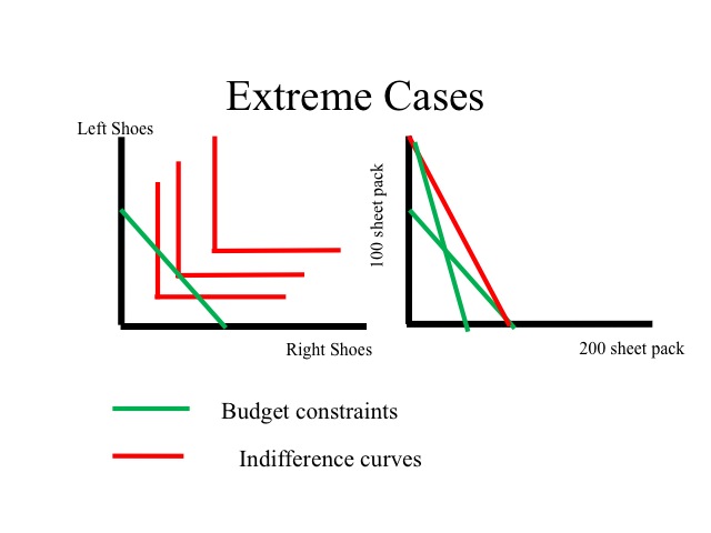
When examining indifference curves and budget constraints, we can look at a few extremes. One extreme case would be if the two goods are perfect complements. For example, you do not get additional satisfaction from having another right shoe, unless you have a left shoe to go with it. In the case of perfect complements, you always consume at the minimum combination of the two goods.
Another extreme is perfect substitutes. You purchase paper in either the 100 or 200 sheet packs and only value the number of sheets. You are indifferent between having two one-hundred sheet packages or one two-hundred sheet package. In the case of perfect substitutes, there are three different outcomes that will maximize utility. If the price of one package, yields a lower per sheet cost, the consumer will buy only that good, so consumption will take place at one of the two intercepts. The third outcome is when the budget constraint has the same slope as the indifference curve. In this case, any combination along the budget constraint will yield the same level of utility.
Government Food Stamps Example
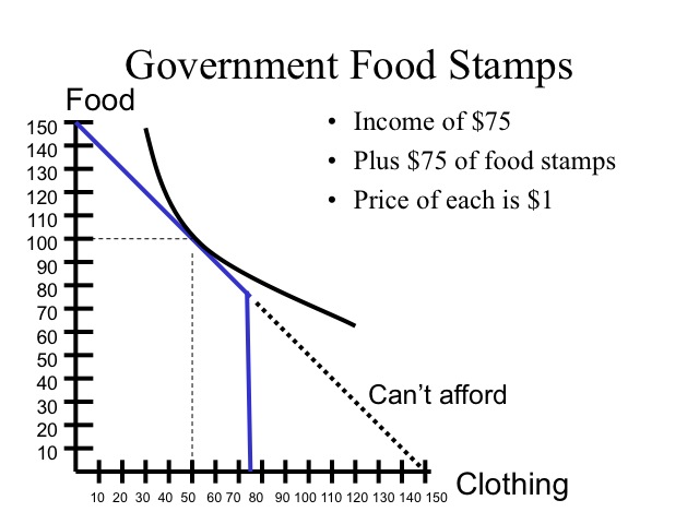
Why does the government give welfare recipients food stamps instead of cash? Why are food stamps sold on the black market for a discount? Let’s assume a person has $75 of income and receives $75 of food stamps from the government. For simplicity, we will assume that the price of each unit of food and the price of clothing are each one dollar. The budget constraint allows the consumer to purchase up to 150 units of food, but since food stamps can only be used to purchase food, the consumer is limited to only being able to purchase 75 units of other items.
The amount of food and other goods, the individual will purchase depends on the shape of his indifference curve. Provided that the person spends at least 75 dollars on food, he is not constrained by receiving food stamps instead of cash.
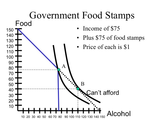
Unfortunately, for those individuals with strong addictions, such as cigarettes or alcohol, their indifference curves reflect the greater value received from the addict substance. Since food stamps only apply to purchasing food, the consumer is not able to get as much utility and is restricted to point A. If the food stamps had been in the form of cash, the consumer would have purchased 40 units of food and 110 units of alcohol, point B, which would yield a higher level of utility.
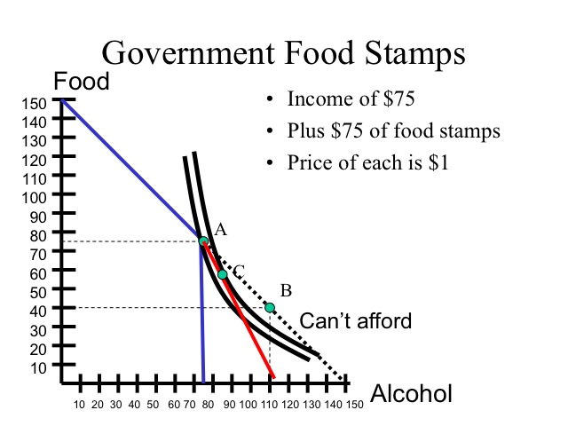
If the consumer could convert a portion of the food stamps to cash, even at a discount, he would be able to reach a higher indifference curve. Assume that he can trade food stamps on the black market for 50 cents on the dollar which extends his budget constraint increasing the amount of alcohol that can be purchased. Selling food stamps at a discount allows the consumer to move to point C, which yields a higher utility than point A.
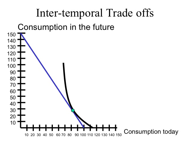
We can also model why individuals purchase items today and carry the debt on their credit cards paying a high interest rate. For example, let’s say the price of each good is $1. Assume Will has $100 of income which he could spend today or invest the money and receive $150 in the future. By waiting, Will would have a greater purchasing power, but his consumption bundle will depend on his preferences. If he has a strong preference for having consumption today, he would be willing to pay a higher price for those goods today. The same is true for those who buy items on credit. They are willing to pay the purchase price plus all the interest, so that they can have it today (so the indifference curve touches the budget constraint at a point closer to the x-axis as seen in the figure).
Similarly, some individuals are willing to pay to go to the expensive theaters to see a movie when it is first released. Others will wait until it comes to the cheap theaters or even until it comes out on DVD/Blu-ray. Although individuals are paying for the “movie experience” and not just the film itself, we can see the time preferences of individuals and the price differentials over time (as represented by different placements of the indifference curves).
